


One-Way ANOVA Test in R
- What is one-way ANOVA test?
- Assumptions of ANOVA test
- How one-way ANOVA test works?
- Visualize your data and compute one-way ANOVA in R
- Summary
- See also
- Read more
- Infos
What is one-way ANOVA test?
ANOVA test hypotheses:
- Null hypothesis: the means of the different groups are the same
- Alternative hypothesis: At least one sample mean is not equal to the others.
Note that, if you have only two groups, you can use t-test. In this case the F-test and the t-test are equivalent.
Assumptions of ANOVA test
Here we describe the requirement for ANOVA test. ANOVA test can be applied only when:
- The observations are obtained independently and randomly from the population defined by the factor levels
- The data of each factor level are normally distributed.
- These normal populations have a common variance. (Levene’s test can be used to check this.)
How one-way ANOVA test works?
Assume that we have 3 groups (A, B, C) to compare:
- Compute the common variance, which is called variance within samples (\(S^2_{within}\)) or residual variance.
- Compute the variance between sample means as follow:
- Compute the mean of each group
- Compute the variance between sample means (\(S^2_{between}\))
- Produce F-statistic as the ratio of \(S^2_{between}/S^2_{within}\).
Note that, a lower ratio (ratio < 1) indicates that there are no significant difference between the means of the samples being compared. However, a higher ratio implies that the variation among group means are significant.
Visualize your data and compute one-way ANOVA in R
Import your data into R
Prepare your data as specified here: Best practices for preparing your data set for R
Save your data in an external .txt tab or .csv files
Import your data into R as follow:
# If .txt tab file, use this
my_data <- read.delim(file.choose())
# Or, if .csv file, use this
my_data <- read.csv(file.choose())
Here, we’ll use the built-in R data set named PlantGrowth. It contains the weight of plants obtained under a control and two different treatment conditions.
my_data <- PlantGrowthCheck your data
To have an idea of what the data look like, we use the the function sample_n()[in dplyr package]. The sample_n() function randomly picks a few of the observations in the data frame to print out:
# Show a random sample
set.seed(1234)
dplyr::sample_n(my_data, 10)
weight group
19 4.32 trt1
18 4.89 trt1
29 5.80 trt2
24 5.50 trt2
17 6.03 trt1
1 4.17 ctrl
6 4.61 ctrl
16 3.83 trt1
12 4.17 trt1
15 5.87 trt1In R terminology, the column “group” is called factor and the different categories (“ctr”, “trt1”, “trt2”) are named factor levels. The levels are ordered alphabetically.
# Show the levels
levels(my_data$group)
[1] "ctrl" "trt1" "trt2"If the levels are not automatically in the correct order, re-order them as follow:
my_data$group <- ordered(my_data$group,
                         levels = c("ctrl", "trt1", "trt2"))
It’s possible to compute summary statistics (mean and sd) by groups using the dplyr package.
- Compute summary statistics by groups - count, mean, sd:
library(dplyr)
group_by(my_data, group) %>%
  summarise(
    count = n(),
    mean = mean(weight, na.rm = TRUE),
    sd = sd(weight, na.rm = TRUE)
  )
Source: local data frame [3 x 4]
group count mean sd
(fctr) (int) (dbl) (dbl)
1 ctrl 10 5.032 0.5830914
2 trt1 10 4.661 0.7936757
3 trt2 10 5.526 0.4425733Visualize your data
To use R base graphs read this: R base graphs. Here, we’ll use the ggpubr R package for an easy ggplot2-based data visualization.
Install the latest version of ggpubr from GitHub as follow (recommended):
# Install
if(!require(devtools)) install.packages("devtools")
devtools::install_github("kassambara/ggpubr")- Or, install from CRAN as follow:
install.packages("ggpubr")- Visualize your data with ggpubr:
# Box plots
# ++++++++++++++++++++
# Plot weight by group and color by group
library("ggpubr")
ggboxplot(my_data, x = "group", y = "weight",
          color = "group", palette = c("#00AFBB", "#E7B800", "#FC4E07"),
          order = c("ctrl", "trt1", "trt2"),
          ylab = "Weight", xlab = "Treatment")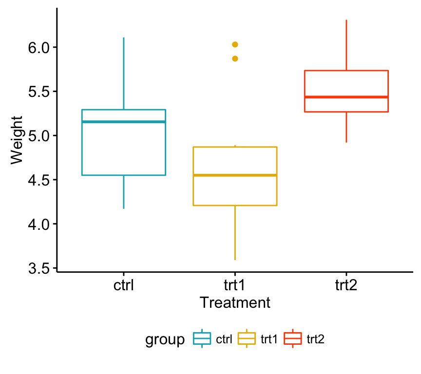
One-way ANOVA Test in R
# Mean plots
# ++++++++++++++++++++
# Plot weight by group
# Add error bars: mean_se
# (other values include: mean_sd, mean_ci, median_iqr, ....)
library("ggpubr")
ggline(my_data, x = "group", y = "weight",
       add = c("mean_se", "jitter"),
       order = c("ctrl", "trt1", "trt2"),
       ylab = "Weight", xlab = "Treatment")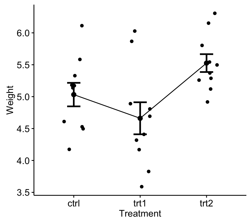
One-way ANOVA Test in R
If you still want to use R base graphs, type the following scripts:
# Box plot
boxplot(weight ~ group, data = my_data,
        xlab = "Treatment", ylab = "Weight",
        frame = FALSE, col = c("#00AFBB", "#E7B800", "#FC4E07"))
# plotmeans
library("gplots")
plotmeans(weight ~ group, data = my_data, frame = FALSE,
          xlab = "Treatment", ylab = "Weight",
          main="Mean Plot with 95% CI")
Compute one-way ANOVA test
We want to know if there is any significant difference between the average weights of plants in the 3 experimental conditions.
The R function aov() can be used to answer to this question. The function summary.aov() is used to summarize the analysis of variance model.
# Compute the analysis of variance
res.aov <- aov(weight ~ group, data = my_data)
# Summary of the analysis
summary(res.aov)
Df Sum Sq Mean Sq F value Pr(>F)
group 2 3.766 1.8832 4.846 0.0159 *
Residuals 27 10.492 0.3886
---
Signif. codes: 0 '***' 0.001 '**' 0.01 '*' 0.05 '.' 0.1 ' ' 1The output includes the columns F value and Pr(>F) corresponding to the p-value of the test.
Interpret the result of one-way ANOVA tests
As the p-value is less than the significance level 0.05, we can conclude that there are significant differences between the groups highlighted with “*" in the model summary.
Multiple pairwise-comparison between the means of groups
In one-way ANOVA test, a significant p-value indicates that some of the group means are different, but we don’t know which pairs of groups are different.
It’s possible to perform multiple pairwise-comparison, to determine if the mean difference between specific pairs of group are statistically significant.
Tukey multiple pairwise-comparisons
As the ANOVA test is significant, we can compute Tukey HSD (Tukey Honest Significant Differences, R function: TukeyHSD()) for performing multiple pairwise-comparison between the means of groups.
The function TukeyHD() takes the fitted ANOVA as an argument.
TukeyHSD(res.aov) Tukey multiple comparisons of means
95% family-wise confidence level
Fit: aov(formula = weight ~ group, data = my_data)
$group
diff lwr upr p adj
trt1-ctrl -0.371 -1.0622161 0.3202161 0.3908711
trt2-ctrl 0.494 -0.1972161 1.1852161 0.1979960
trt2-trt1 0.865 0.1737839 1.5562161 0.0120064- diff: difference between means of the two groups
- lwr, upr: the lower and the upper end point of the confidence interval at 95% (default)
- p adj: p-value after adjustment for the multiple comparisons.
It can be seen from the output, that only the difference between trt2 and trt1 is significant with an adjusted p-value of 0.012.
Multiple comparisons using multcomp package
It’s possible to use the function glht() [in multcomp package] to perform multiple comparison procedures for an ANOVA. glht stands for general linear hypothesis tests. The simplified format is as follow:
glht(model, lincft)- model: a fitted model, for example an object returned by aov().
- lincft(): a specification of the linear hypotheses to be tested. Multiple comparisons in ANOVA models are specified by objects returned from the function mcp().
Use glht() to perform multiple pairwise-comparisons for a one-way ANOVA:
library(multcomp)
summary(glht(res.aov, linfct = mcp(group = "Tukey")))
     Simultaneous Tests for General Linear Hypotheses
Multiple Comparisons of Means: Tukey Contrasts
Fit: aov(formula = weight ~ group, data = my_data)
Linear Hypotheses:
                 Estimate Std. Error t value Pr(>|t|)
trt1 - ctrl == 0  -0.3710     0.2788  -1.331    0.391
trt2 - ctrl == 0   0.4940     0.2788   1.772    0.198
trt2 - trt1 == 0   0.8650     0.2788   3.103    0.012 *
---
Signif. codes:  0 '***' 0.001 '**' 0.01 '*' 0.05 '.' 0.1 ' ' 1
(Adjusted p values reported -- single-step method)
Pairewise t-test
The function pairewise.t.test() can be also used to calculate pairwise comparisons between group levels with corrections for multiple testing.
pairwise.t.test(my_data$weight, my_data$group,
                 p.adjust.method = "BH")
    Pairwise comparisons using t tests with pooled SD
data:  my_data$weight and my_data$group
     ctrl  trt1
trt1 0.194 -
trt2 0.132 0.013
P value adjustment method: BH
The result is a table of p-values for the pairwise comparisons. Here, the p-values have been adjusted by the Benjamini-Hochberg method.
Check ANOVA assumptions: test validity?
The ANOVA test assumes that, the data are normally distributed and the variance across groups are homogeneous. We can check that with some diagnostic plots.
Check the homogeneity of variance assumption
The residuals versus fits plot can be used to check the homogeneity of variances.
In the plot below, there is no evident relationships between residuals and fitted values (the mean of each groups), which is good. So, we can assume the homogeneity of variances.
# 1. Homogeneity of variances
plot(res.aov, 1)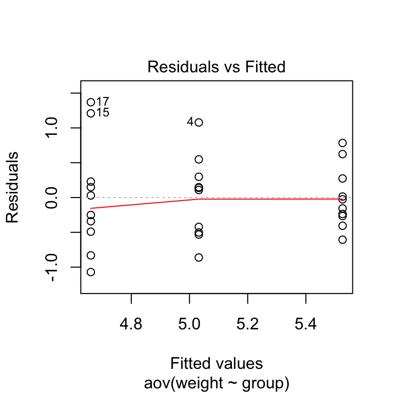
One-way ANOVA Test in R
Points 17, 15, 4 are detected as outliers, which can severely affect normality and homogeneity of variance. It can be useful to remove outliers to meet the test assumptions.
It’s also possible to use Bartlett’s test or Levene’s test to check the homogeneity of variances.
We recommend Levene’s test, which is less sensitive to departures from normal distribution. The function leveneTest() [in car package] will be used:
library(car)
leveneTest(weight ~ group, data = my_data)
Levene's Test for Homogeneity of Variance (center = median)
Df F value Pr(>F)
group 2 1.1192 0.3412
27 From the output above we can see that the p-value is not less than the significance level of 0.05. This means that there is no evidence to suggest that the variance across groups is statistically significantly different. Therefore, we can assume the homogeneity of variances in the different treatment groups.
Relaxing the homogeneity of variance assumption
The classical one-way ANOVA test requires an assumption of equal variances for all groups. In our example, the homogeneity of variance assumption turned out to be fine: the Levene test is not significant.
How do we save our ANOVA test, in a situation where the homogeneity of variance assumption is violated?
An alternative procedure (i.e.: Welch one-way test), that does not require that assumption have been implemented in the function oneway.test().
- ANOVA test with no assumption of equal variances
oneway.test(weight ~ group, data = my_data)- Pairwise t-tests with no assumption of equal variances
pairwise.t.test(my_data$weight, my_data$group,
                 p.adjust.method = "BH", pool.sd = FALSE)
Check the normality assumption
Normality plot of residuals. In the plot below, the quantiles of the residuals are plotted against the quantiles of the normal distribution. A 45-degree reference line is also plotted.
The normal probability plot of residuals is used to check the assumption that the residuals are normally distributed. It should approximately follow a straight line.
# 2. Normality
plot(res.aov, 2)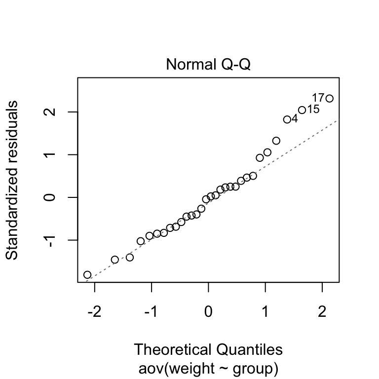
One-way ANOVA Test in R
As all the points fall approximately along this reference line, we can assume normality.
The conclusion above, is supported by the Shapiro-Wilk test on the ANOVA residuals (W = 0.96, p = 0.6) which finds no indication that normality is violated.
# Extract the residuals
aov_residuals <- residuals(object = res.aov )
# Run Shapiro-Wilk test
shapiro.test(x = aov_residuals )
    Shapiro-Wilk normality test
data:  aov_residuals
W = 0.96607, p-value = 0.4379
Non-parametric alternative to one-way ANOVA test
Note that, a non-parametric alternative to one-way ANOVA is Kruskal-Wallis rank sum test, which can be used when ANNOVA assumptions are not met.
kruskal.test(weight ~ group, data = my_data)
    Kruskal-Wallis rank sum test
data:  weight by group
Kruskal-Wallis chi-squared = 7.9882, df = 2, p-value = 0.01842
Summary
- Import your data from a .txt tab file: my_data <- read.delim(file.choose()). Here, we used my_data <- PlantGrowth.
- Visualize your data: ggpubr::ggboxplot(my_data, x = “group”, y = “weight”, color = “group”)
- Compute one-way ANOVA test: summary(aov(weight ~ group, data = my_data))
- Tukey multiple pairwise-comparisons: TukeyHSD(res.aov)
See also
- Analysis of variance (ANOVA, parametric):
- Kruskal-Wallis Test in R (non parametric alternative to one-way ANOVA)
Read more
- (Quick-R: ANOVA/MANOVA)[http://www.statmethods.net/stats/anova.html]
- (Quick-R: (M)ANOVA Assumptions)[http://www.statmethods.net/stats/anovaAssumptions.html]
- (R and Analysis of Variance)[http://personality-project.org/r/r.guide/r.anova.html
Infos
This analysis has been performed using R software (ver. 3.2.4).
Show me some love with the like buttons below... Thank you and please don't forget to share and comment below!!
Montrez-moi un peu d'amour avec les like ci-dessous ... Merci et n'oubliez pas, s'il vous plaît, de partager et de commenter ci-dessous!
Recommended for You!


Recommended for you
This section contains best data science and self-development resources to help you on your path.
Coursera - Online Courses and Specialization
Data science
- Course: Machine Learning: Master the Fundamentals by Standford
- Specialization: Data Science by Johns Hopkins University
- Specialization: Python for Everybody by University of Michigan
- Courses: Build Skills for a Top Job in any Industry by Coursera
- Specialization: Master Machine Learning Fundamentals by University of Washington
- Specialization: Statistics with R by Duke University
- Specialization: Software Development in R by Johns Hopkins University
- Specialization: Genomic Data Science by Johns Hopkins University
Popular Courses Launched in 2020
- Google IT Automation with Python by Google
- AI for Medicine by deeplearning.ai
- Epidemiology in Public Health Practice by Johns Hopkins University
- AWS Fundamentals by Amazon Web Services
Trending Courses
- The Science of Well-Being by Yale University
- Google IT Support Professional by Google
- Python for Everybody by University of Michigan
- IBM Data Science Professional Certificate by IBM
- Business Foundations by University of Pennsylvania
- Introduction to Psychology by Yale University
- Excel Skills for Business by Macquarie University
- Psychological First Aid by Johns Hopkins University
- Graphic Design by Cal Arts
Books - Data Science
Our Books
- Practical Guide to Cluster Analysis in R by A. Kassambara (Datanovia)
- Practical Guide To Principal Component Methods in R by A. Kassambara (Datanovia)
- Machine Learning Essentials: Practical Guide in R by A. Kassambara (Datanovia)
- R Graphics Essentials for Great Data Visualization by A. Kassambara (Datanovia)
- GGPlot2 Essentials for Great Data Visualization in R by A. Kassambara (Datanovia)
- Network Analysis and Visualization in R by A. Kassambara (Datanovia)
- Practical Statistics in R for Comparing Groups: Numerical Variables by A. Kassambara (Datanovia)
- Inter-Rater Reliability Essentials: Practical Guide in R by A. Kassambara (Datanovia)
Others
- R for Data Science: Import, Tidy, Transform, Visualize, and Model Data by Hadley Wickham & Garrett Grolemund
- Hands-On Machine Learning with Scikit-Learn, Keras, and TensorFlow: Concepts, Tools, and Techniques to Build Intelligent Systems by Aurelien Géron
- Practical Statistics for Data Scientists: 50 Essential Concepts by Peter Bruce & Andrew Bruce
- Hands-On Programming with R: Write Your Own Functions And Simulations by Garrett Grolemund & Hadley Wickham
- An Introduction to Statistical Learning: with Applications in R by Gareth James et al.
- Deep Learning with R by François Chollet & J.J. Allaire
- Deep Learning with Python by François Chollet