survminer 0.3.0

Release notes

In this post, we present only the most important changes in v0.3.0. See the release notes for a complete list.

Installing and loading survminer

Install the latest developmental version from GitHub:

if(!require(devtools)) install.packages("devtools")
devtools::install_github("kassambara/survminer", build_vignettes = TRUE)

Or, install the latest release from CRAN as follow:

install.packages("survminer")

To load survminer in R, type this:

library("survminer")

Survival curves

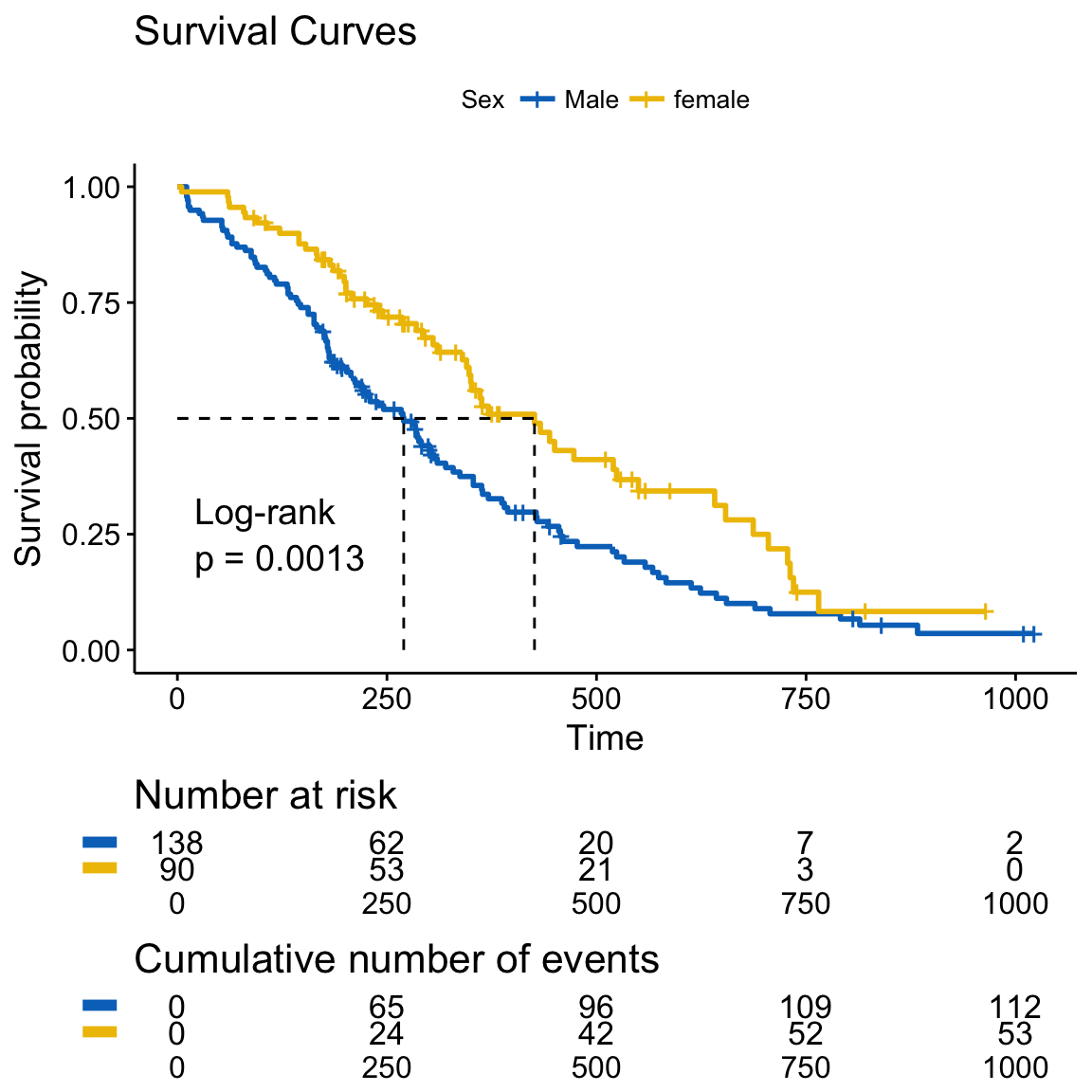
New arguments displaying supplementary survival tables - cumulative events & censored subjects - under the main survival curves:

# Fit survival curves
require("survival")
fit <- survfit(Surv(time, status) ~ sex, data = lung)
# Plot informative survival curves
library("survminer")
ggsurvplot(fit, data = lung,
           title = "Survival Curves",
           pval = TRUE, pval.method = TRUE,    # Add p-value &  method name
           surv.median.line = "hv",            # Add median survival lines
           legend.title = "Sex",               # Change legend titles
           legend.labs = c("Male", "female"),  # Change legend labels
           palette = "jco",                    # Use JCO journal color palette
           risk.table = TRUE,                  # Add No at risk table
           cumevents = TRUE,                   # Add cumulative No of events table
           tables.height = 0.15,               # Specify tables height
           tables.theme = theme_cleantable(),  # Clean theme for tables
           tables.y.text = FALSE               # Hide tables y axis text
)

survminer

Cumulative events and censored tables are good additional feedback to survival curves, so that one could realize: what is the number of risk set AND what is the cause that the risk set become smaller: is it caused by events or by censored events?

Arranging multiple ggsurvplots on the same page

The function arrange_ggsurvplots() [in survminer] can be used to arrange multiple ggsurvplots on the same page.

# List of ggsurvplots
splots <- list()
splots[[1]] <- ggsurvplot(fit, data = lung,
                          risk.table = TRUE,
                          tables.y.text = FALSE,
                          ggtheme = theme_light())
splots[[2]] <- ggsurvplot(fit, data = lung,
                          risk.table = TRUE,
                          tables.y.text = FALSE,
                          ggtheme = theme_grey())
# Arrange multiple ggsurvplots and print the output
arrange_ggsurvplots(splots, print = TRUE,
  ncol = 2, nrow = 1, risk.table.height = 0.25)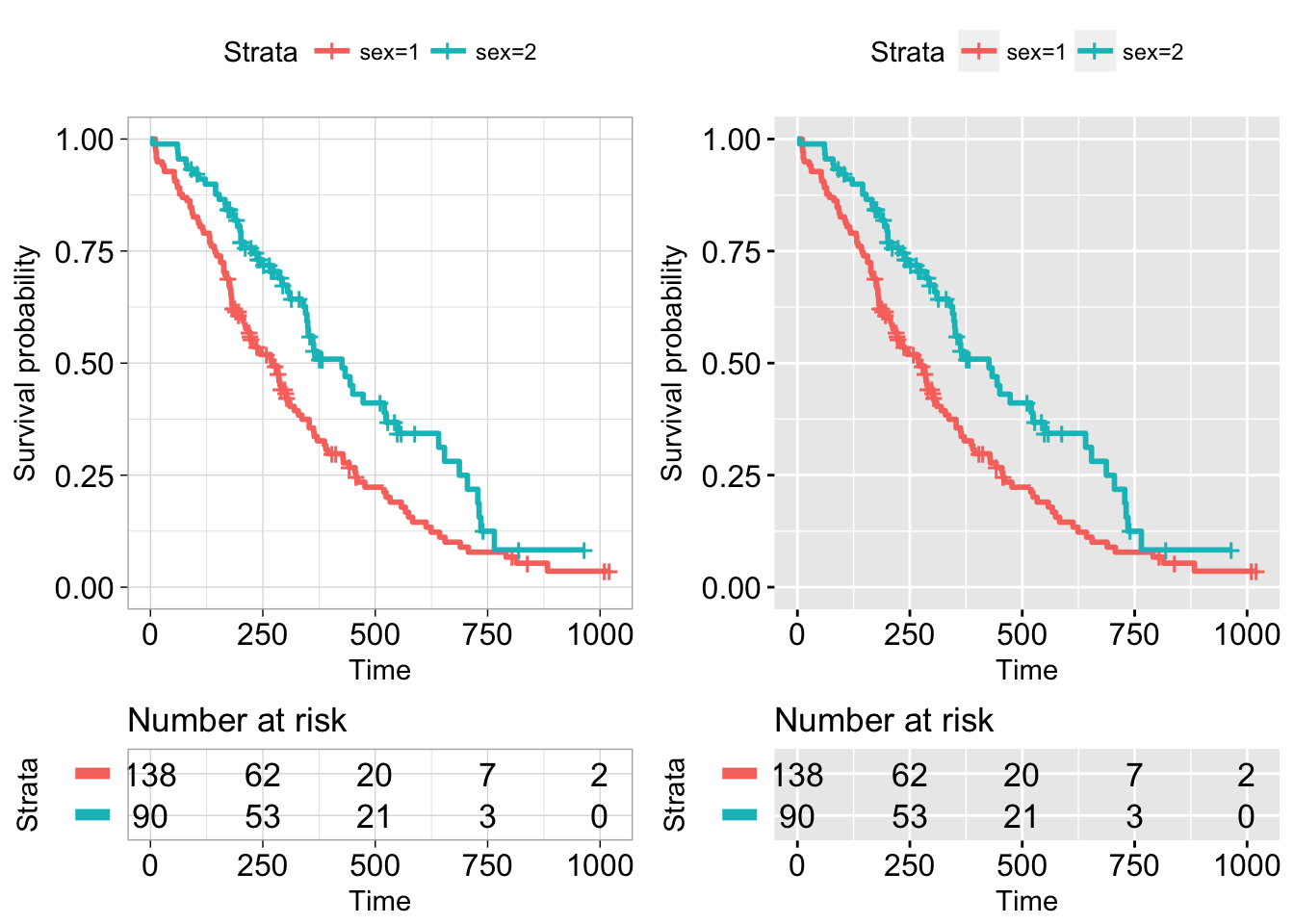

survminer

If you want to save the output into a pdf, type this:

# Arrange and save into pdf file
res <- arrange_ggsurvplots(splots, print = FALSE)
ggsave("myfile.pdf", res)

Distribution of events’ times

The function ggsurvevents() [in survminer] calculates and plots the distribution for events (both status = 0 and status = 1). It helps to notice when censoring is more common (@pbiecek, #116). This is an alternative to cumulative events and censored tables, described in the previous section.

For example in colon dataset, as illustrated below, censoring occur mostly after the 6’th year:

require("survival")
surv <- Surv(colon$time, colon$status)
ggsurvevents(surv)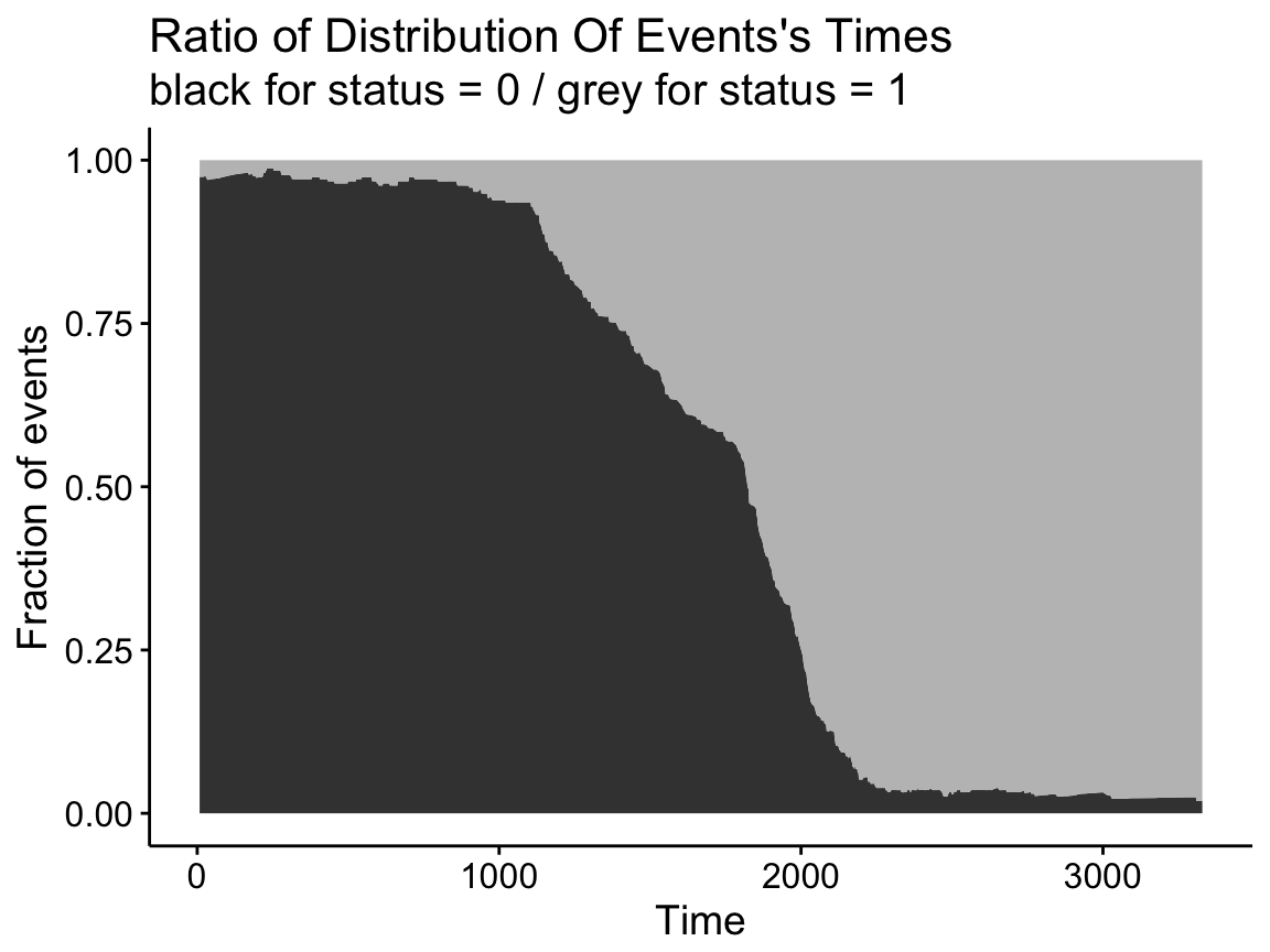

survminer

Adjusted survival curves for Cox model

Adjusted survival curves show how a selected factor influences survival estimated from a cox model. If you want read more about why we need to adjust survival curves, see this document: Adjusted survival curves.

Briefly, in clinical investigations, there are many situations, where several known factors, potentially affect patient prognosis. For example, suppose two groups of patients are compared: those with and those without a specific genotype. If one of the groups also contains older individuals, any difference in survival may be attributable to genotype or age or indeed both. Hence, when investigating survival in relation to any one factor, it is often desirable to adjust for the impact of others.

The cox proportional-hazards model is one of the most important methods used for modelling survival analysis data.

Here, we present the function ggcoxadjustedcurves() [in survminer] for plotting adjusted survival curves for cox proportional hazards model. The ggcoxadjustedcurves() function models the risks due to the confounders as described in the section 5.2 of this article: Terry M Therneau (2015); Adjusted survival curves. Briefly, the key idea is to predict survival for all individuals in the cohort, and then take the average of the predicted curves by groups of interest (for example, sex, age, genotype groups, etc.).

# Data preparation and computing cox model
library(survival)
lung$sex <- factor(lung$sex, levels = c(1,2),
                   labels = c("Male", "Female"))
res.cox <- coxph(Surv(time, status) ~ sex + age + ph.ecog, data =  lung)
# Plot the baseline survival function
# with showing all individual predicted surv. curves
ggcoxadjustedcurves(res.cox, data = lung,
                    individual.curves = TRUE)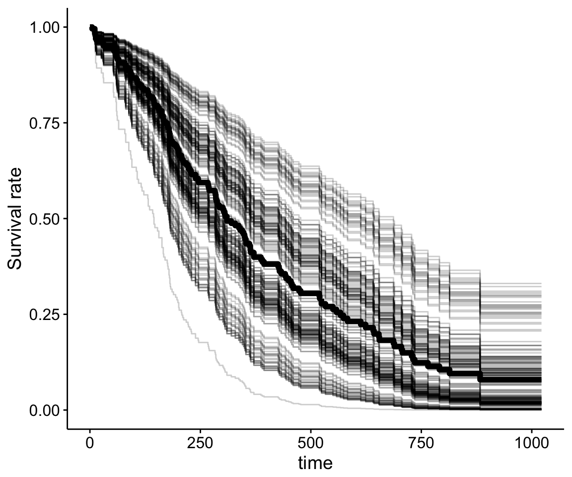

survminer

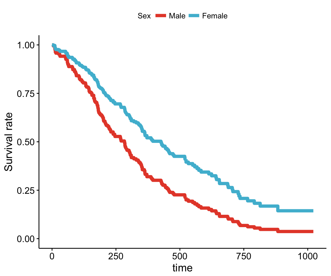
# Adjusted survival curves for the variable "sex"
ggcoxadjustedcurves(res.cox, data = lung,
                   variable  = lung[, "sex"],   # Variable of interest
                   legend.title = "Sex",        # Change legend title
                   palette = "npg",             # nature publishing group color palettes
                   curv.size = 2                # Change line size
                   )

survminer

Graphical summary of Cox model

The function ggforest() [in survminer] can be used to create a graphical summary of a Cox model, also known as forest plot. For each covariate, it displays the hazard ratio (HR) and the 95% confidence intervals of the HR. By default, covariates with significant p-value are highlighted in red.

# Fit a Cox model
library(survival)
res.cox <- coxph(Surv(time, status) ~ sex + age + ph.ecog, data =  lung)
res.cox

## Call:
## coxph(formula = Surv(time, status) ~ sex + age + ph.ecog, data = lung)
##
##               coef exp(coef) se(coef)     z       p
## sexFemale -0.55261   0.57544  0.16774 -3.29 0.00099
## age        0.01107   1.01113  0.00927  1.19 0.23242
## ph.ecog    0.46373   1.58999  0.11358  4.08 4.4e-05
##
## Likelihood ratio test=30.5  on 3 df, p=1.08e-06
## n= 227, number of events= 164
##    (1 observation deleted due to missingness)

# Create a forest plot
ggforest(res.cox)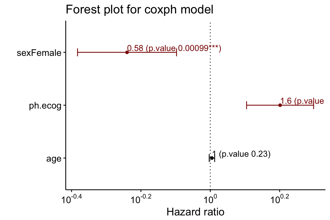

survminer

Pairwise comparisons for survival curves

When you compare three or more survival curves at once, the function survdiff() [in survival package] returns a global p-value whether to reject or not the null hypothesis.

With this, you know that a difference exists between groups, but you don’t know where. You can’t know until you test each combination.

Therefore, we implemented the function pairwise_survdiff() [in survminer]. It calculates pairwise comparisons between group levels with corrections for multiple testing.

• Multiple survival curves with global p-value:

library("survival")
library("survminer")
# Survival curves with global p-value
data(myeloma)
fit2 <- survfit(Surv(time, event) ~ molecular_group, data = myeloma)
ggsurvplot(fit2, data = myeloma,
           legend.title = "Molecular Group",
           legend.labs = levels(myeloma$molecular_group),
           legend = "right",
           pval = TRUE, palette = "lancet")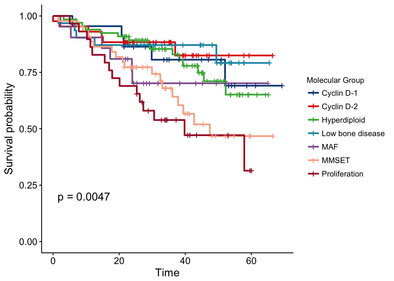

survminer

• Pairwise survdiff:

# Pairwise survdiff
res <- pairwise_survdiff(Surv(time, event) ~ molecular_group,
     data = myeloma)
res

##
##  Pairwise comparisons using Log-Rank test
##
## data:  myeloma and molecular_group
##
##                  Cyclin D-1 Cyclin D-2 Hyperdiploid Low bone disease MAF   MMSET
## Cyclin D-2       0.723      -          -            -                -     -
## Hyperdiploid     0.328      0.103      -            -                -     -
## Low bone disease 0.644      0.447      0.723        -                -     -
## MAF              0.943      0.723      0.103        0.523            -     -
## MMSET            0.103      0.038      0.527        0.485            0.038 -
## Proliferation    0.723      0.988      0.103        0.485            0.644 0.062
##
## P value adjustment method: BH

• Symbolic number coding:

# Symbolic number coding
symnum(res$p.value, cutpoints = c(0, 0.0001, 0.001, 0.01, 0.05, 0.1, 1),
   symbols = c("****", "***", "**", "*", "+", " "),
   abbr.colnames = FALSE, na = "")

##                  Cyclin D-1 Cyclin D-2 Hyperdiploid Low bone disease MAF MMSET
## Cyclin D-2
## Hyperdiploid
## Low bone disease
## MAF
## MMSET                       *                                        *
## Proliferation                                                            +
## attr(,"legend")
## [1] 0 '****' 1e-04 '***' 0.001 '**' 0.01 '*' 0.05 '+' 0.1 ' ' 1 \t    ## NA: ''

Visualizing competing risk analysis

Competing risk events refer to a situation where an individual (patient) is at risk of more than one mutually exclusive event, such as death from different causes, and the occurrence of one of these will prevent any other event from ever happening.

For example, when studying relapse in patients who underwent HSCT (Hematopoietic stem cell transplantation), transplant related mortality is a competing risk event and the cumulative incidence function (CIF) must be calculated by appropriate accounting.

A ‘competing risks’ analysis is implemented in the R package cmprsk. Here, we provide the ggcompetingrisks() function [in survminer] to plot the results using ggplot2-based elegant data visualization.

# Create a demo data set
#%%%%%%%%%%%%%%%%%%%%%%%%%%%%%%%%%%%
set.seed(2)
failure_time <- rexp(100)
status <- factor(sample(0:2, 100, replace=TRUE), 0:2,
                 c('no event', 'death', 'progression'))
disease <- factor(sample(1:3,  100,replace=TRUE), 1:3,
                  c('BRCA','LUNG','OV'))
# Cumulative Incidence Function
#%%%%%%%%%%%%%%%%%%%%%%%%%%%%%%
require(cmprsk)
fit3 <- cuminc(ftime = failure_time, fstatus = status,
              group = disease)
# Visualize
#%%%%%%%%%%%%%%%%%%%%%%%%%%%%%
ggcompetingrisks(fit3, palette = "Dark2",
                 legend = "top",
                 ggtheme = theme_bw())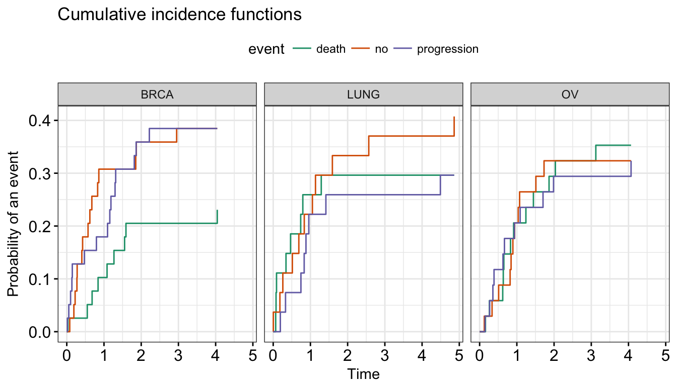

survminer

The ggcometingrisks() function has also support for multi-state survival objects (type = “mstate”), where the status variable can have multiple levels. The first of these will stand for censoring, and the others for various event types, e.g., causes of death.

# Data preparation
df <- data.frame(time = failure_time, status = status,
                 group = disease)
# Fit multi-state survival
library(survival)
fit5 <- survfit(Surv(time, status, type = "mstate") ~ group, data = df)
ggcompetingrisks(fit5, palette = "jco")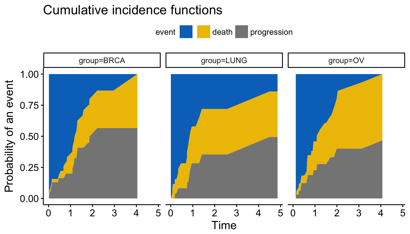

survminer

Related articles

• Survival Analysis
  • Survival Analysis Basics: Curves and Logrank Tests
  • Cox Proportional Hazards Model
  • Cox Model Assumptions

Infos

This analysis has been performed using R software (ver. 3.3.2).

Recommended for you