


Cox Proportional-Hazards Model
The Cox proportional-hazards model (Cox, 1972) is essentially a regression model commonly used statistical in medical research for investigating the association between the survival time of patients and one or more predictor variables.
In the previous chapter (survival analysis basics), we described the basic concepts of survival analyses and methods for analyzing and summarizing survival data, including:
- the definition of hazard and survival functions,
- the construction of Kaplan-Meier survival curves for different patient groups
- the logrank test for comparing two or more survival curves
The above mentioned methods - Kaplan-Meier curves and logrank tests - are examples of univariate analysis. They describe the survival according to one factor under investigation, but ignore the impact of any others.
Additionally, Kaplan-Meier curves and logrank tests are useful only when the predictor variable is categorical (e.g.: treatment A vs treatment B; males vs females). They don’t work easily for quantitative predictors such as gene expression, weight, or age.
An alternative method is the Cox proportional hazards regression analysis, which works for both quantitative predictor variables and for categorical variables. Furthermore, the Cox regression model extends survival analysis methods to assess simultaneously the effect of several risk factors on survival time.
In this article, we’ll describe the Cox regression model and provide practical examples using R software.
The need for multivariate statistical modeling
In clinical investigations, there are many situations, where several known quantities (known as covariates), potentially affect patient prognosis.
For instance, suppose two groups of patients are compared: those with and those without a specific genotype. If one of the groups also contains older individuals, any difference in survival may be attributable to genotype or age or indeed both. Hence, when investigating survival in relation to any one factor, it is often desirable to adjust for the impact of others.
Statistical model is a frequently used tool that allows to analyze survival with respect to several factors simultaneously. Additionally, statistical model provides the effect size for each factor.
The cox proportional-hazards model is one of the most important methods used for modelling survival analysis data. The next section introduces the basics of the Cox regression model.
Basics of the Cox proportional hazards model
The purpose of the model is to evaluate simultaneously the effect of several factors on survival. In other words, it allows us to examine how specified factors influence the rate of a particular event happening (e.g., infection, death) at a particular point in time. This rate is commonly referred as the hazard rate. Predictor variables (or factors) are usually termed covariates in the survival-analysis literature.
The Cox model is expressed by the hazard function denoted by h(t). Briefly, the hazard function can be interpreted as the risk of dying at time t. It can be estimated as follow:
\[ h(t) = h_0(t) \times exp(b_1x_1 + b_2x_2 + ... + b_px_p) \]
where,
- t represents the survival time
- \(h(t)\) is the hazard function determined by a set of p covariates (\(x_1, x_2, ..., x_p\))
- the coefficients (\(b_1, b_2, ..., b_p\)) measure the impact (i.e., the effect size) of covariates.
- the term \(h_0\) is called the baseline hazard. It corresponds to the value of the hazard if all the \(x_i\) are equal to zero (the quantity exp(0) equals 1). The ‘t’ in h(t) reminds us that the hazard may vary over time.
The Cox model can be written as a multiple linear regression of the logarithm of the hazard on the variables \(x_i\), with the baseline hazard being an ‘intercept’ term that varies with time.
The quantities \(exp(b_i)\) are called hazard ratios (HR). A value of \(b_i\) greater than zero, or equivalently a hazard ratio greater than one, indicates that as the value of the \(i^{th}\) covariate increases, the event hazard increases and thus the length of survival decreases.
Put another way, a hazard ratio above 1 indicates a covariate that is positively associated with the event probability, and thus negatively associated with the length of survival.
In summary,
- HR = 1: No effect
- HR < 1: Reduction in the hazard
- HR > 1: Increase in Hazard
Note that in cancer studies:
- A covariate with hazard ratio > 1 (i.e.: b > 0) is called bad prognostic factor
- A covariate with hazard ratio < 1 (i.e.: b < 0) is called good prognostic factor
A key assumption of the Cox model is that the hazard curves for the groups of observations (or patients) should be proportional and cannot cross.
Consider two patients k and k’ that differ in their x-values. The corresponding hazard function can be simply written as follow
- Hazard function for the patient k:
\[ h_k(t) = h_0(t)e^{\sum\limits_{i=1}^n{\beta x}} \]
- Hazard function for the patient k’:
\[ h_{k'}(t) = h_0(t)e^{\sum\limits_{i=1}^n{\beta x'}} \]
- The hazard ratio for these two patients [\(\frac{h_k(t)}{h_{k'}(t)} = \frac{h_0(t)e^{\sum\limits_{i=1}^n{\beta x}}}{h_0(t)e^{\sum\limits_{i=1}^n{\beta x'}}} = \frac{e^{\sum\limits_{i=1}^n{\beta x}}}{e^{\sum\limits_{i=1}^n{\beta x'}}}\)] is independent of time t.
Consequently, the Cox model is a proportional-hazards model: the hazard of the event in any group is a constant multiple of the hazard in any other. This assumption implies that, as mentioned above, the hazard curves for the groups should be proportional and cannot cross.
In other words, if an individual has a risk of death at some initial time point that is twice as high as that of another individual, then at all later times the risk of death remains twice as high.
This assumption of proportional hazards should be tested. We’ll discuss methods for assessing proportionality in the next article in this series: Cox Model Assumptions.
Compute the Cox model in R
Install and load required R package
We’ll use two R packages:
- survival for computing survival analyses
survminer for visualizing survival analysis results
Install the packages
install.packages(c("survival", "survminer"))- Load the packages
library("survival")
library("survminer")
R function to compute the Cox model: coxph()
The function coxph()[in survival package] can be used to compute the Cox proportional hazards regression model in R.
The simplified format is as follow:
coxph(formula, data, method)- formula: is linear model with a survival object as the response variable. Survival object is created using the function Surv() as follow: Surv(time, event).
- data: a data frame containing the variables
- method: is used to specify how to handle ties. The default is ‘efron’. Other options are ‘breslow’ and ‘exact’. The default ‘efron’ is generally preferred to the once-popular “breslow” method. The “exact” method is much more computationally intensive.
Example data sets
We’ll use the lung cancer data in the survival R package.
data("lung")
head(lung)
inst time status age sex ph.ecog ph.karno pat.karno meal.cal wt.loss
1 3 306 2 74 1 1 90 100 1175 NA
2 3 455 2 68 1 0 90 90 1225 15
3 3 1010 1 56 1 0 90 90 NA 15
4 5 210 2 57 1 1 90 60 1150 11
5 1 883 2 60 1 0 100 90 NA 0
6 12 1022 1 74 1 1 50 80 513 0- inst: Institution code
- time: Survival time in days
- status: censoring status 1=censored, 2=dead
- age: Age in years
- sex: Male=1 Female=2
- ph.ecog: ECOG performance score (0=good 5=dead)
- ph.karno: Karnofsky performance score (bad=0-good=100) rated by physician
- pat.karno: Karnofsky performance score as rated by patient
- meal.cal: Calories consumed at meals
- wt.loss: Weight loss in last six months
Compute the Cox model
We’ll fit the Cox regression using the following covariates: age, sex, ph.ecog and wt.loss.
We start by computing univariate Cox analyses for all these variables; then we’ll fit multivariate cox analyses using two variables to describe how the factors jointly impact on survival.
Univariate Cox regression
Univariate Cox analyses can be computed as follow:
res.cox <- coxph(Surv(time, status) ~ sex, data = lung)
res.cox
Call:
coxph(formula = Surv(time, status) ~ sex, data = lung)
coef exp(coef) se(coef) z p
sex -0.531 0.588 0.167 -3.18 0.0015
Likelihood ratio test=10.6 on 1 df, p=0.00111
n= 228, number of events= 165 The function summary() for Cox models produces a more complete report:
summary(res.cox)Call:
coxph(formula = Surv(time, status) ~ sex, data = lung)
n= 228, number of events= 165
coef exp(coef) se(coef) z Pr(>|z|)
sex -0.5310 0.5880 0.1672 -3.176 0.00149 **
---
Signif. codes: 0 '***' 0.001 '**' 0.01 '*' 0.05 '.' 0.1 ' ' 1
exp(coef) exp(-coef) lower .95 upper .95
sex 0.588 1.701 0.4237 0.816
Concordance= 0.579 (se = 0.022 )
Rsquare= 0.046 (max possible= 0.999 )
Likelihood ratio test= 10.63 on 1 df, p=0.001111
Wald test = 10.09 on 1 df, p=0.001491
Score (logrank) test = 10.33 on 1 df, p=0.001312The Cox regression results can be interpreted as follow:
Statistical significance. The column marked “z” gives the Wald statistic value. It corresponds to the ratio of each regression coefficient to its standard error (z = coef/se(coef)). The wald statistic evaluates, whether the beta (\(\beta\)) coefficient of a given variable is statistically significantly different from 0. From the output above, we can conclude that the variable sex have highly statistically significant coefficients.
The regression coefficients. The second feature to note in the Cox model results is the the sign of the regression coefficients (coef). A positive sign means that the hazard (risk of death) is higher, and thus the prognosis worse, for subjects with higher values of that variable. The variable sex is encoded as a numeric vector. 1: male, 2: female. The R summary for the Cox model gives the hazard ratio (HR) for the second group relative to the first group, that is, female versus male. The beta coefficient for sex = -0.53 indicates that females have lower risk of death (lower survival rates) than males, in these data.
Hazard ratios. The exponentiated coefficients (exp(coef) = exp(-0.53) = 0.59), also known as hazard ratios, give the effect size of covariates. For example, being female (sex=2) reduces the hazard by a factor of 0.59, or 41%. Being female is associated with good prognostic.
Confidence intervals of the hazard ratios. The summary output also gives upper and lower 95% confidence intervals for the hazard ratio (exp(coef)), lower 95% bound = 0.4237, upper 95% bound = 0.816.
Global statistical significance of the model. Finally, the output gives p-values for three alternative tests for overall significance of the model: The likelihood-ratio test, Wald test, and score logrank statistics. These three methods are asymptotically equivalent. For large enough N, they will give similar results. For small N, they may differ somewhat. The Likelihood ratio test has better behavior for small sample sizes, so it is generally preferred.
To apply the univariate coxph function to multiple covariates at once, type this:
covariates <- c("age", "sex",  "ph.karno", "ph.ecog", "wt.loss")
univ_formulas <- sapply(covariates,
                        function(x) as.formula(paste('Surv(time, status)~', x)))

univ_models <- lapply( univ_formulas, function(x){coxph(x, data = lung)})
# Extract data
univ_results <- lapply(univ_models,
                       function(x){
                          x <- summary(x)
                          p.value<-signif(x$wald["pvalue"], digits=2)
                          wald.test<-signif(x$wald["test"], digits=2)
                          beta<-signif(x$coef[1], digits=2);#coeficient beta
                          HR <-signif(x$coef[2], digits=2);#exp(beta)
                          HR.confint.lower <- signif(x$conf.int[,"lower .95"], 2)
                          HR.confint.upper <- signif(x$conf.int[,"upper .95"],2)
                          HR <- paste0(HR, " (",
                                       HR.confint.lower, "-", HR.confint.upper, ")")
                          res<-c(beta, HR, wald.test, p.value)
                          names(res)<-c("beta", "HR (95% CI for HR)", "wald.test",
                                        "p.value")
                          return(res)
                          #return(exp(cbind(coef(x),confint(x))))
                         })
res <- t(as.data.frame(univ_results, check.names = FALSE))
as.data.frame(res)
beta HR (95% CI for HR) wald.test p.value
age 0.019 1 (1-1) 4.1 0.042
sex -0.53 0.59 (0.42-0.82) 10 0.0015
ph.karno -0.016 0.98 (0.97-1) 7.9 0.005
ph.ecog 0.48 1.6 (1.3-2) 18 2.7e-05
wt.loss 0.0013 1 (0.99-1) 0.05 0.83The output above shows the regression beta coefficients, the effect sizes (given as hazard ratios) and statistical significance for each of the variables in relation to overall survival. Each factor is assessed through separate univariate Cox regressions.
From the output above,
The variables sex, age and ph.ecog have highly statistically significant coefficients, while the coefficient for ph.karno is not significant.
age and ph.ecog have positive beta coefficients, while sex has a negative coefficient. Thus, older age and higher ph.ecog are associated with poorer survival, whereas being female (sex=2) is associated with better survival.
Now, we want to describe how the factors jointly impact on survival. To answer to this question, we’ll perform a multivariate Cox regression analysis. As the variable ph.karno is not significant in the univariate Cox analysis, we’ll skip it in the multivariate analysis. We’ll include the 3 factors (sex, age and ph.ecog) into the multivariate model.
Multivariate Cox regression analysis
A Cox regression of time to death on the time-constant covariates is specified as follow:
res.cox <- coxph(Surv(time, status) ~ age + sex + ph.ecog, data =  lung)
summary(res.cox)
Call:
coxph(formula = Surv(time, status) ~ age + sex + ph.ecog, data = lung)
n= 227, number of events= 164
(1 observation deleted due to missingness)
coef exp(coef) se(coef) z Pr(>|z|)
age 0.011067 1.011128 0.009267 1.194 0.232416
sex -0.552612 0.575445 0.167739 -3.294 0.000986 ***
ph.ecog 0.463728 1.589991 0.113577 4.083 4.45e-05 ***
---
Signif. codes: 0 '***' 0.001 '**' 0.01 '*' 0.05 '.' 0.1 ' ' 1
exp(coef) exp(-coef) lower .95 upper .95
age 1.0111 0.9890 0.9929 1.0297
sex 0.5754 1.7378 0.4142 0.7994
ph.ecog 1.5900 0.6289 1.2727 1.9864
Concordance= 0.637 (se = 0.026 )
Rsquare= 0.126 (max possible= 0.999 )
Likelihood ratio test= 30.5 on 3 df, p=1.083e-06
Wald test = 29.93 on 3 df, p=1.428e-06
Score (logrank) test = 30.5 on 3 df, p=1.083e-06The p-value for all three overall tests (likelihood, Wald, and score) are significant, indicating that the model is significant. These tests evaluate the omnibus null hypothesis that all of the betas (\(\beta\)) are 0. In the above example, the test statistics are in close agreement, and the omnibus null hypothesis is soundly rejected.
In the multivariate Cox analysis, the covariates sex and ph.ecog remain significant (p < 0.05). However, the covariate age fails to be significant (p = 0.23, which is grater than 0.05).
The p-value for sex is 0.000986, with a hazard ratio HR = exp(coef) = 0.58, indicating a strong relationship between the patients’ sex and decreased risk of death. The hazard ratios of covariates are interpretable as multiplicative effects on the hazard. For example, holding the other covariates constant, being female (sex=2) reduces the hazard by a factor of 0.58, or 42%. We conclude that, being female is associated with good prognostic.
Similarly, the p-value for ph.ecog is 4.45e-05, with a hazard ratio HR = 1.59, indicating a strong relationship between the ph.ecog value and increased risk of death. Holding the other covariates constant, a higher value of ph.ecog is associated with a poor survival.
By contrast, the p-value for age is now p=0.23. The hazard ratio HR = exp(coef) = 1.01, with a 95% confidence interval of 0.99 to 1.03. Because the confidence interval for HR includes 1, these results indicate that age makes a smaller contribution to the difference in the HR after adjusting for the ph.ecog values and patient’s sex, and only trend toward significance. For example, holding the other covariates constant, an additional year of age induce daily hazard of death by a factor of exp(beta) = 1.01, or 1%, which is not a significant contribution.
Visualizing the estimated distribution of survival times
Having fit a Cox model to the data, it’s possible to visualize the predicted survival proportion at any given point in time for a particular risk group. The function survfit() estimates the survival proportion, by default at the mean values of covariates.
# Plot the baseline survival function
ggsurvplot(survfit(res.cox), color = "#2E9FDF",
           ggtheme = theme_minimal())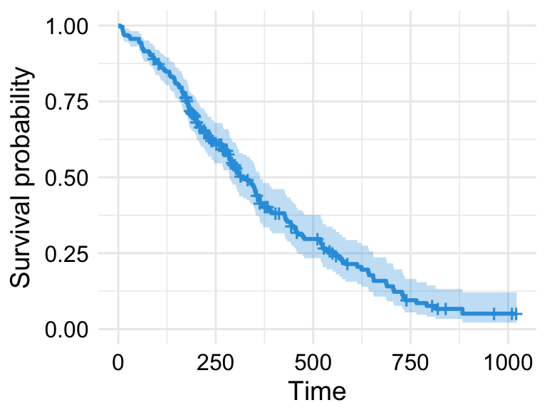
Cox Proportional-Hazards Model
We may wish to display how estimated survival depends upon the value of a covariate of interest.
Consider that, we want to assess the impact of the sex on the estimated survival probability. In this case, we construct a new data frame with two rows, one for each value of sex; the other covariates are fixed to their average values (if they are continuous variables) or to their lowest level (if they are discrete variables). For a dummy covariate, the average value is the proportion coded 1 in the data set. This data frame is passed to survfit() via the newdata argument:
# Create the new data
sex_df <- with(lung,
               data.frame(sex = c(1, 2),
                          age = rep(mean(age, na.rm = TRUE), 2),
                          ph.ecog = c(1, 1)
                          )
               )
sex_df
sex age ph.ecog
1 1 62.44737 1
2 2 62.44737 1# Survival curves
fit <- survfit(res.cox, newdata = sex_df)
ggsurvplot(fit, conf.int = TRUE, legend.labs=c("Sex=1", "Sex=2"),
ggtheme = theme_minimal())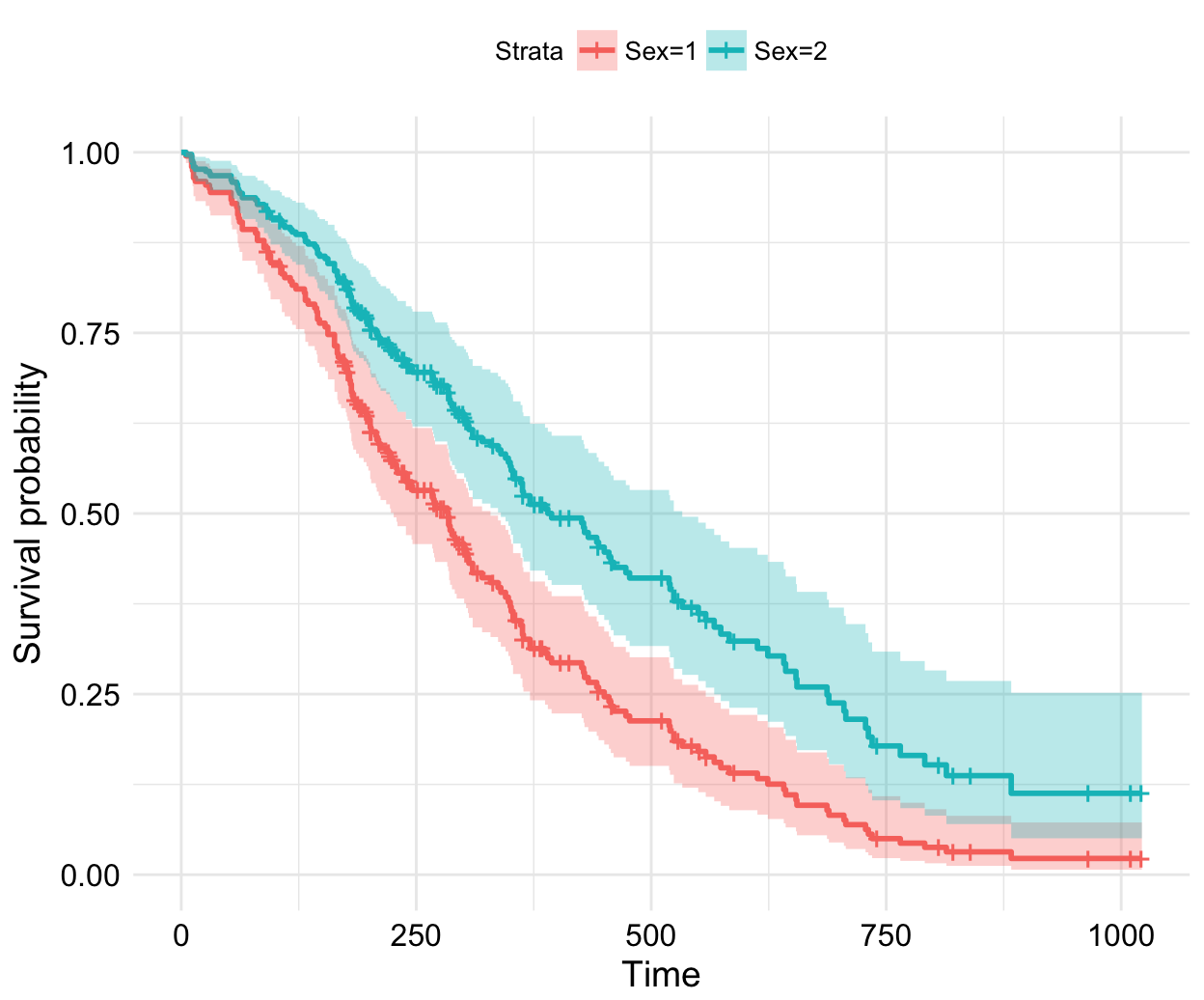
Cox Proportional-Hazards Model
Summary
In this article, we described the Cox regression model for assessing simultaneously the relationship between multiple risk factors and patient’s survival time. We demonstrated how to compute the Cox model using the survival package. Additionally, we described how to visualize the results of the analysis using the survminer package.
References
- Cox DR (1972). Regression models and life tables (with discussion). J R Statist Soc B 34: 187–220
- MJ Bradburn, TG Clark, SB Love and DG Altman. Survival Analysis Part II: Multivariate data analysis – an introduction to concepts and methods. British Journal of Cancer (2003) 89, 431 – 436
Infos
This analysis has been performed using R software (ver. 3.3.2).
Show me some love with the like buttons below... Thank you and please don't forget to share and comment below!!
Montrez-moi un peu d'amour avec les like ci-dessous ... Merci et n'oubliez pas, s'il vous plaît, de partager et de commenter ci-dessous!
Recommended for You!


Recommended for you
This section contains best data science and self-development resources to help you on your path.
Coursera - Online Courses and Specialization
Data science
- Course: Machine Learning: Master the Fundamentals by Standford
- Specialization: Data Science by Johns Hopkins University
- Specialization: Python for Everybody by University of Michigan
- Courses: Build Skills for a Top Job in any Industry by Coursera
- Specialization: Master Machine Learning Fundamentals by University of Washington
- Specialization: Statistics with R by Duke University
- Specialization: Software Development in R by Johns Hopkins University
- Specialization: Genomic Data Science by Johns Hopkins University
Popular Courses Launched in 2020
- Google IT Automation with Python by Google
- AI for Medicine by deeplearning.ai
- Epidemiology in Public Health Practice by Johns Hopkins University
- AWS Fundamentals by Amazon Web Services
Trending Courses
- The Science of Well-Being by Yale University
- Google IT Support Professional by Google
- Python for Everybody by University of Michigan
- IBM Data Science Professional Certificate by IBM
- Business Foundations by University of Pennsylvania
- Introduction to Psychology by Yale University
- Excel Skills for Business by Macquarie University
- Psychological First Aid by Johns Hopkins University
- Graphic Design by Cal Arts
Books - Data Science
Our Books
- Practical Guide to Cluster Analysis in R by A. Kassambara (Datanovia)
- Practical Guide To Principal Component Methods in R by A. Kassambara (Datanovia)
- Machine Learning Essentials: Practical Guide in R by A. Kassambara (Datanovia)
- R Graphics Essentials for Great Data Visualization by A. Kassambara (Datanovia)
- GGPlot2 Essentials for Great Data Visualization in R by A. Kassambara (Datanovia)
- Network Analysis and Visualization in R by A. Kassambara (Datanovia)
- Practical Statistics in R for Comparing Groups: Numerical Variables by A. Kassambara (Datanovia)
- Inter-Rater Reliability Essentials: Practical Guide in R by A. Kassambara (Datanovia)
Others
- R for Data Science: Import, Tidy, Transform, Visualize, and Model Data by Hadley Wickham & Garrett Grolemund
- Hands-On Machine Learning with Scikit-Learn, Keras, and TensorFlow: Concepts, Tools, and Techniques to Build Intelligent Systems by Aurelien Géron
- Practical Statistics for Data Scientists: 50 Essential Concepts by Peter Bruce & Andrew Bruce
- Hands-On Programming with R: Write Your Own Functions And Simulations by Garrett Grolemund & Hadley Wickham
- An Introduction to Statistical Learning: with Applications in R by Gareth James et al.
- Deep Learning with R by François Chollet & J.J. Allaire
- Deep Learning with Python by François Chollet