Read counting - NGS

Introduction

We will describe how to count next generation sequencing reads, which fall into genomic features. The result is a count matrix which has rows corresponding to genomic ranges and columns which correspond to different experiments or samples.

As an example, we will use an RNA-Seq experiment, with files in the `pasillaBamSubset` Bioconductor data package. However, the same functions can be used for DNA-Seq and ChIP-Seq.

Load transcript database

#source("http://bioconductor.org/biocLite.R")
#biocLite("pasillaBamSubset")
#biocLite("TxDb.Dmelanogaster.UCSC.dm3.ensGene")
library(pasillaBamSubset)
library(TxDb.Dmelanogaster.UCSC.dm3.ensGene)

We load a transcript database object. These are prebuilt in R for various well studied organisms, for example TxDb.Hsapiens.UCSC.hg19.knownGene. In addition the makeTranscriptDbFromGFF file can be used to import GFF or GTF gene models. We use the exonsBy function to get a GRangesList object of the exons for each gene.

#Rename the transcript database
txdb <- TxDb.Dmelanogaster.UCSC.dm3.ensGene
#For each gene pull up the exons
grl <- exonsBy(txdb, by="gene")
#exons of the 100th gene
grl[100]

## GRangesList of length 1:
## $FBgn0000286 
## GRanges with 8 ranges and 2 metadata columns:
##       seqnames             ranges strand |   exon_id   exon_name
##                       |  
##   [1]    chr2L [4876890, 4879196]      - |      8515        
##   [2]    chr2L [4877289, 4879196]      - |      8516        
##   [3]    chr2L [4880294, 4880472]      - |      8517        
##   [4]    chr2L [4880378, 4880472]      - |      8518        
##   [5]    chr2L [4881215, 4882492]      - |      8519        
##   [6]    chr2L [4882865, 4883113]      - |      8520        
##   [7]    chr2L [4882889, 4883113]      - |      8521        
##   [8]    chr2L [4882889, 4883341]      - |      8522        
## 
## ---
## seqlengths:
##      chr2L     chr2R     chr3L     chr3R      chr4      chrX ...  chr3LHet  chr3RHet   chrXHet   chrYHet chrUextra
##   23011544  21146708  24543557  27905053   1351857  22422827 ...   2555491   2517507    204112    347038  29004656

grl[[100]]

## GRanges with 8 ranges and 2 metadata columns:
##       seqnames             ranges strand |   exon_id   exon_name
##                       |  
##   [1]    chr2L [4876890, 4879196]      - |      8515        
##   [2]    chr2L [4877289, 4879196]      - |      8516        
##   [3]    chr2L [4880294, 4880472]      - |      8517        
##   [4]    chr2L [4880378, 4880472]      - |      8518        
##   [5]    chr2L [4881215, 4882492]      - |      8519        
##   [6]    chr2L [4882865, 4883113]      - |      8520        
##   [7]    chr2L [4882889, 4883113]      - |      8521        
##   [8]    chr2L [4882889, 4883341]      - |      8522        
##   ---
##   seqlengths:
##        chr2L     chr2R     chr3L     chr3R      chr4      chrX ...  chr3LHet  chr3RHet   chrXHet   chrYHet chrUextra
##     23011544  21146708  24543557  27905053   1351857  22422827 ...   2555491   2517507    204112    347038  29004656

grl[[100]][1]#first exon of the 100th gene

## GRanges with 1 range and 2 metadata columns:
##       seqnames             ranges strand |   exon_id   exon_name
##                       |  
##   [1]    chr2L [4876890, 4879196]      - |      8515        
##   ---
##   seqlengths:
##        chr2L     chr2R     chr3L     chr3R      chr4      chrX ...  chr3LHet  chr3RHet   chrXHet   chrYHet chrUextra
##     23011544  21146708  24543557  27905053   1351857  22422827 ...   2555491   2517507    204112    347038  29004656

Load bam files

These functions in the pasillaBamSubset package just point us to the BAM files.

fl1 <- untreated1_chr4()
fl2 <- untreated3_chr4()
fl1

## [1] "/Library/Frameworks/R.framework/Versions/3.1/Resources/library/pasillaBamSubset/extdata/untreated1_chr4.bam"

Read counting in bam files

We need the following libraries for counting BAM files.

library(Rsamtools)
library(GenomicRanges)

Note: if you are using Bioconductor version 14, paired with R 3.1, you should also load this library. You do not need to load this library, and it will not be available to you, if you are using Bioconductor version 13, paired with R 3.0.x.

#Required for Bioc 14 and R 3.1
library(GenomicAlignments)

We specify the files using the BamFileList function. This allows us to tell the read counting functions how many reads to load at once. For larger files, yield size of 1 million reads might make sense.

The yield size is how many reads that we want to pull from each bam file.

fls <- BamFileList(c(fl1, fl2), yieldSize=5e4)
names(fls) <- c("first","second")

The following function counts the overlaps of the reads in the BAM files in the features, which are the genes of Drosophila. We tell the counting function to ignore the strand, i.e., to allow minus strand reads to count in plus strand genes, and vice versa.

so1 <- summarizeOverlaps(features=grl,
                         reads=fls,
                         ignore.strand=TRUE)
#summarized experiment
#The rowData contains information about the features
#and the colData contains information about the files which we specified.
so1

## class: SummarizedExperiment 
## dim: 15682 2 
## exptData(0):
## assays(1): counts
## rownames(15682): FBgn0000003 FBgn0000008 ... FBgn0264726 FBgn0264727
## rowData metadata column names(0):
## colnames(2): first second
## colData names(0):

Others important parameters of summarizeOverlaps are : inter.feature: default is true. We are only interested in counting reads which uniquely align to one feature. singleEnd : default is true. Which says that these files have single-end reads instead of paired-end reads. fragments : If you are counting reads in a paired-end experiment, it’s specifying that you also want to count reads where only one of the two reads in a pair aligns.

We can examine the count matrix, which is stored in the assay slot:

head(assay(so1))

##             first second
## FBgn0000003     0      0
## FBgn0000008     0      0
## FBgn0000014     0      0
## FBgn0000015     0      0
## FBgn0000017     0      0
## FBgn0000018     0      0

#sum of the count matrix
#number of reads which aligned-- uniquely-- to these features.
colSums(assay(so1))

##  first second 
## 156469 122872

#Information about the features (genes)
rowData(so1)

## GRangesList of length 15682:
## $FBgn0000003 
## GRanges with 1 range and 2 metadata columns:
##       seqnames             ranges strand |   exon_id   exon_name
##                       |  
##   [1]    chr3R [2648220, 2648518]      + |     45123        
## 
## $FBgn0000008 
## GRanges with 13 ranges and 2 metadata columns:
##        seqnames               ranges strand   | exon_id exon_name
##    [1]    chr2R [18024494, 18024531]      +   |   20314      
##    [2]    chr2R [18024496, 18024713]      +   |   20315      
##    [3]    chr2R [18024938, 18025756]      +   |   20316      
##    [4]    chr2R [18025505, 18025756]      +   |   20317      
##    [5]    chr2R [18039159, 18039200]      +   |   20322      
##    ...      ...                  ...    ... ...     ...       ...
##    [9]    chr2R [18058283, 18059490]      +   |   20326      
##   [10]    chr2R [18059587, 18059757]      +   |   20327      
##   [11]    chr2R [18059821, 18059938]      +   |   20328      
##   [12]    chr2R [18060002, 18060339]      +   |   20329      
##   [13]    chr2R [18060002, 18060346]      +   |   20330      
## 
## ...
## <15680 more elements>
## ---
## seqlengths:
##      chr2L     chr2R     chr3L     chr3R      chr4      chrX ...  chr3LHet  chr3RHet   chrXHet   chrYHet chrUextra
##   23011544  21146708  24543557  27905053   1351857  22422827 ...   2555491   2517507    204112    347038  29004656

#Information about the samples (here it's empty)
colData(so1)

## DataFrame with 2 rows and 0 columns

#add information (sample columns)
colData(so1)$sample <- c("one","two")
colData(so1)

## DataFrame with 2 rows and 1 column
##             sample
##        
## first          one
## second         two

#metadata  information on the features
#It tells you information which is how this row data was generated.
#It was generated from a transcriptDb using the genomic features package.
#The data source was UCSC, the genome was dm3, the organism was drosphila, etc.
#pretty useful for reproducibility of count tables.
metadata(rowData(so1))

## $genomeInfo
## $genomeInfo$`Db type`
## [1] "TranscriptDb"
## 
## $genomeInfo$`Supporting package`
## [1] "GenomicFeatures"
## 
## $genomeInfo$`Data source`
## [1] "UCSC"
## 
## $genomeInfo$Genome
## [1] "dm3"
## 
## $genomeInfo$Organism
## [1] "Drosophila melanogaster"
## 
## $genomeInfo$`UCSC Table`
## [1] "ensGene"
## 
## $genomeInfo$`Resource URL`
## [1] "http://genome.ucsc.edu/"
## 
## $genomeInfo$`Type of Gene ID`
## [1] "Ensembl gene ID"
## 
## $genomeInfo$`Full dataset`
## [1] "yes"
## 
## $genomeInfo$`miRBase build ID`
## [1] NA
## 
## $genomeInfo$transcript_nrow
## [1] "29173"
## 
## $genomeInfo$exon_nrow
## [1] "76920"
## 
## $genomeInfo$cds_nrow
## [1] "62135"
## 
## $genomeInfo$`Db created by`
## [1] "GenomicFeatures package from Bioconductor"
## 
## $genomeInfo$`Creation time`
## [1] "2014-03-17 16:24:54 -0700 (Mon, 17 Mar 2014)"
## 
## $genomeInfo$`GenomicFeatures version at creation time`
## [1] "1.15.11"
## 
## $genomeInfo$`RSQLite version at creation time`
## [1] "0.11.4"
## 
## $genomeInfo$DBSCHEMAVERSION
## [1] "1.0"

Exploratory data analysis of the counts:

x <- assay(so1)[,1]
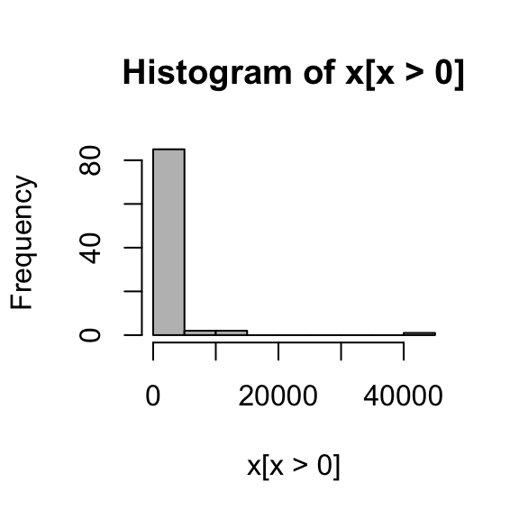
hist(x[x > 0], col="grey")
#We can see that there's at least one very, very large count here (more than 40,000).
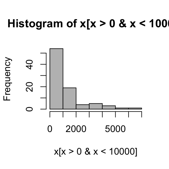
#if we exclude accounts over 10,000, we can see a bit more of the distribution.
hist(x[x > 0 & x < 10000], col="grey")
#Scatterplot of the 2 samples in log scale
plot(assay(so1) + 1, log="xy")# +1 to avoid log (0)

The second file should actually be counted in a special manner, as it contains pairs of reads which come from a single fragment. We do not want to count these twice, so we set singleEnd = FALSE. Additionally, we specify fragments = TRUE which counts reads if only one of the pair aligns to the features, and the other pair aligns to no feature.

# ?untreated3_chr4
# ?summarizeOverlaps
fls <- BamFileList(fl2, yieldSize=5e4)
so2 <- summarizeOverlaps(features=grl,
                         reads=fls,
                         ignore.strand=TRUE,
                         singleEnd=FALSE, 
                         fragments=TRUE)#if only one of a pair of reads maps, we also want to count this.
#we can look at the number of reads which align this time.
#And we can note that the last time, when we count each read alone, we had about two times more reads.
#So 60,000 to 120,000.
colSums(assay(so2))

## untreated3_chr4.bam 
##               65591

colSums(assay(so1))

##  first second 
## 156469 122872

plot(assay(so1)[,2], assay(so2)[,1], xlim=c(0,5000), ylim=c(0,5000),
     xlab="single end counting", ylab="paired end counting")
abline(0,1)
abline(0,.5)

scatter plot: when we counted each read singly and we counted only pairs. If you make a y equals x plot line and a y equals 1/2 x line, you can see essentially these counts are about half, because when we did the single-end counting, we were counting each read instead of each fragment.

Footnotes

Licence

Licence

References

https://github.com/genomicsclass

Recommended for you