


One-Sample T-test in R
- What is one-sample t-test?
- Research questions and statistical hypotheses
- Formula of one-sample t-test
- Visualize your data and compute one-sample t-test in R
- Install ggpubr R package for data visualization
- R function to compute one-sample t-test
- Import your data into R
- Check your data
- Visualize your data using box plots
- Preleminary test to check one-sample t-test assumptions
- Compute one-sample t-test
- Interpretation of the result
- Access to the values returned by t.test() function
- Online one-sample t-test calculator
- See also
- Infos
What is one-sample t-test?
Generally, the theoretical mean comes from:
- a previous experiment. For example, compare whether the mean weight of mice differs from 200 mg, a value determined in a previous study.
- or from an experiment where you have control and treatment conditions. If you express your data as “percent of control”, you can test whether the average value of treatment condition differs significantly from 100.
Note that, one-sample t-test can be used only, when the data are normally distributed . This can be checked using Shapiro-Wilk test .
Research questions and statistical hypotheses
Typical research questions are:
- whether the mean (\(m\)) of the sample is equal to the theoretical mean (\(\mu\))?
- whether the mean (\(m\)) of the sample is less than the theoretical mean (\(\mu\))?
- whether the mean (\(m\)) of the sample is greater than the theoretical mean (\(\mu\))?
In statistics, we can define the corresponding null hypothesis (\(H_0\)) as follow:
- \(H_0: m = \mu\)
- \(H_0: m \leq \mu\)
- \(H_0: m \geq \mu\)
The corresponding alternative hypotheses (\(H_a\)) are as follow:
- \(H_a: m \ne \mu\) (different)
- \(H_a: m > \mu\) (greater)
- \(H_a: m < \mu\) (less)
Note that:
- Hypotheses 1) are called two-tailed tests
- Hypotheses 2) and 3) are called one-tailed tests
Formula of one-sample t-test
The t-statistic can be calculated as follow:
\[ t = \frac{m-\mu}{s/\sqrt{n}} \]
where,
- m is the sample mean
- n is the sample size
- s is the sample standard deviation with \(n-1\) degrees of freedom
- \(\mu\) is the theoretical value
We can compute the p-value corresponding to the absolute value of the t-test statistics (|t|) for the degrees of freedom (df): \(df = n - 1\).
How to interpret the results?
If the p-value is inferior or equal to the significance level 0.05, we can reject the null hypothesis and accept the alternative hypothesis. In other words, we conclude that the sample mean is significantly different from the theoretical mean.
Visualize your data and compute one-sample t-test in R
Install ggpubr R package for data visualization
You can draw R base graps as described at this link: R base graphs. Here, we’ll use the ggpubr R package for an easy ggplot2-based data visualization
- Install the latest version from GitHub as follow (recommended):
# Install
if(!require(devtools)) install.packages("devtools")
devtools::install_github("kassambara/ggpubr")- Or, install from CRAN as follow:
install.packages("ggpubr")R function to compute one-sample t-test
To perform one-sample t-test, the R function t.test() can be used as follow:
t.test(x, mu = 0, alternative = "two.sided")- x: a numeric vector containing your data values
- mu: the theoretical mean. Default is 0 but you can change it.
- alternative: the alternative hypothesis. Allowed value is one of “two.sided” (default), “greater” or “less”.
Import your data into R
Prepare your data as specified here: Best practices for preparing your data set for R
Save your data in an external .txt tab or .csv files
Import your data into R as follow:
# If .txt tab file, use this
my_data <- read.delim(file.choose())
# Or, if .csv file, use this
my_data <- read.csv(file.choose())
Here, we’ll use an example data set containing the weight of 10 mice.
We want to know, if the average weight of the mice differs from 25g?
set.seed(1234)
my_data <- data.frame(
  name = paste0(rep("M_", 10), 1:10),
  weight = round(rnorm(10, 20, 2), 1)
)
Check your data
# Print the first 10 rows of the data
head(my_data, 10)
name weight
1 M_1 17.6
2 M_2 20.6
3 M_3 22.2
4 M_4 15.3
5 M_5 20.9
6 M_6 21.0
7 M_7 18.9
8 M_8 18.9
9 M_9 18.9
10 M_10 18.2# Statistical summaries of weight
summary(my_data$weight) Min. 1st Qu. Median Mean 3rd Qu. Max.
15.30 18.38 18.90 19.25 20.82 22.20 - Min.: the minimum value
- 1st Qu.: The first quartile. 25% of values are lower than this.
- Median: the median value. Half the values are lower; half are higher.
- 3rd Qu.: the third quartile. 75% of values are higher than this.
- Max.: the maximum value
Visualize your data using box plots
library(ggpubr)
ggboxplot(my_data$weight,
          ylab = "Weight (g)", xlab = FALSE,
          ggtheme = theme_minimal())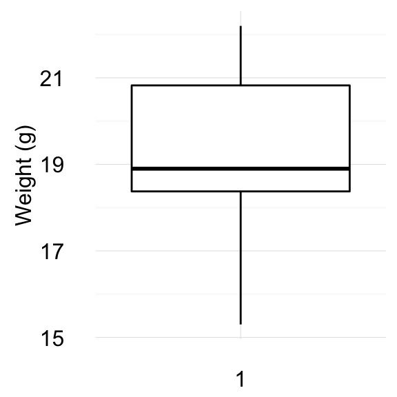
One-Sample Student’s T-test in R
Preleminary test to check one-sample t-test assumptions
- Is this a large sample? - No, because n < 30.
- Since the sample size is not large enough (less than 30, central limit theorem), we need to check whether the data follow a normal distribution.
How to check the normality?
Read this article: Normality Test in R.
Briefly, it’s possible to use the Shapiro-Wilk normality test and to look at the normality plot.
- Shapiro-Wilk test:
- Null hypothesis: the data are normally distributed
- Alternative hypothesis: the data are not normally distributed
shapiro.test(my_data$weight) # => p-value = 0.6993From the output, the p-value is greater than the significance level 0.05 implying that the distribution of the data are not significantly different from normal distribtion. In other words, we can assume the normality.
- Visual inspection of the data normality using Q-Q plots (quantile-quantile plots). Q-Q plot draws the correlation between a given sample and the normal distribution.
library("ggpubr")
ggqqplot(my_data$weight, ylab = "Men's weight",
         ggtheme = theme_minimal())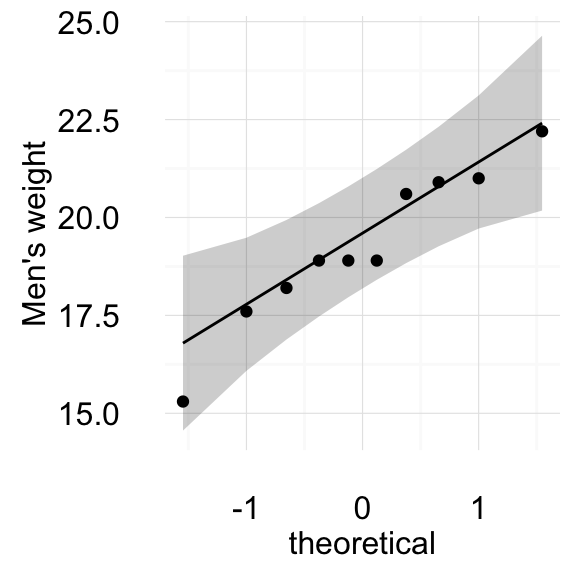
One-Sample Student’s T-test in R
From the normality plots, we conclude that the data may come from normal distributions.
Note that, if the data are not normally distributed, it’s recommended to use the non parametric one-sample Wilcoxon rank test.
Compute one-sample t-test
We want to know, if the average weight of the mice differs from 25g (two-tailed test)?
# One-sample t-test
res <- t.test(my_data$weight, mu = 25)
# Printing the results
res
    One Sample t-test
data:  my_data$weight
t = -9.0783, df = 9, p-value = 7.953e-06
alternative hypothesis: true mean is not equal to 25
95 percent confidence interval:
 17.8172 20.6828
sample estimates:
mean of x
    19.25
In the result above :
- t is the t-test statistic value (t = -9.078),
- df is the degrees of freedom (df= 9),
- p-value is the significance level of the t-test (p-value = 7.95310^{-6}).
- conf.int is the confidence interval of the mean at 95% (conf.int = [17.8172, 20.6828]);
- sample estimates is he mean value of the sample (mean = 19.25).
Note that:
- if you want to test whether the mean weight of mice is less than 25g (one-tailed test), type this:
t.test(my_data$weight, mu = 25,
alternative = "less")- Or, if you want to test whether the mean weight of mice is greater than 25g (one-tailed test), type this:
t.test(my_data$weight, mu = 25,
              alternative = "greater")
Interpretation of the result
The p-value of the test is 7.95310^{-6}, which is less than the significance level alpha = 0.05. We can conclude that the mean weight of the mice is significantly different from 25g with a p-value = 7.95310^{-6}.
Access to the values returned by t.test() function
The result of t.test() function is a list containing the following components:
- statistic: the value of the t test statistics
- parameter: the degrees of freedom for the t test statistics
- p.value: the p-value for the test
- conf.int: a confidence interval for the mean appropriate to the specified alternative hypothesis.
- estimate: the means of the two groups being compared (in the case of independent t test) or difference in means (in the case of paired t test).
The format of the R code to use for getting these values is as follow:
# printing the p-value
res$p.value
[1] 7.953383e-06# printing the mean
res$estimatemean of x
19.25 # printing the confidence interval
res$conf.int[1] 17.8172 20.6828
attr(,"conf.level")
[1] 0.95Online one-sample t-test calculator
You can perform one-sample t-test, online, without any installation by clicking the following link:
Infos
This analysis has been performed using R software (ver. 3.2.4).
Show me some love with the like buttons below... Thank you and please don't forget to share and comment below!!
Montrez-moi un peu d'amour avec les like ci-dessous ... Merci et n'oubliez pas, s'il vous plaît, de partager et de commenter ci-dessous!
Recommended for You!


Recommended for you
This section contains best data science and self-development resources to help you on your path.
Coursera - Online Courses and Specialization
Data science
- Course: Machine Learning: Master the Fundamentals by Standford
- Specialization: Data Science by Johns Hopkins University
- Specialization: Python for Everybody by University of Michigan
- Courses: Build Skills for a Top Job in any Industry by Coursera
- Specialization: Master Machine Learning Fundamentals by University of Washington
- Specialization: Statistics with R by Duke University
- Specialization: Software Development in R by Johns Hopkins University
- Specialization: Genomic Data Science by Johns Hopkins University
Popular Courses Launched in 2020
- Google IT Automation with Python by Google
- AI for Medicine by deeplearning.ai
- Epidemiology in Public Health Practice by Johns Hopkins University
- AWS Fundamentals by Amazon Web Services
Trending Courses
- The Science of Well-Being by Yale University
- Google IT Support Professional by Google
- Python for Everybody by University of Michigan
- IBM Data Science Professional Certificate by IBM
- Business Foundations by University of Pennsylvania
- Introduction to Psychology by Yale University
- Excel Skills for Business by Macquarie University
- Psychological First Aid by Johns Hopkins University
- Graphic Design by Cal Arts
Books - Data Science
Our Books
- Practical Guide to Cluster Analysis in R by A. Kassambara (Datanovia)
- Practical Guide To Principal Component Methods in R by A. Kassambara (Datanovia)
- Machine Learning Essentials: Practical Guide in R by A. Kassambara (Datanovia)
- R Graphics Essentials for Great Data Visualization by A. Kassambara (Datanovia)
- GGPlot2 Essentials for Great Data Visualization in R by A. Kassambara (Datanovia)
- Network Analysis and Visualization in R by A. Kassambara (Datanovia)
- Practical Statistics in R for Comparing Groups: Numerical Variables by A. Kassambara (Datanovia)
- Inter-Rater Reliability Essentials: Practical Guide in R by A. Kassambara (Datanovia)
Others
- R for Data Science: Import, Tidy, Transform, Visualize, and Model Data by Hadley Wickham & Garrett Grolemund
- Hands-On Machine Learning with Scikit-Learn, Keras, and TensorFlow: Concepts, Tools, and Techniques to Build Intelligent Systems by Aurelien Géron
- Practical Statistics for Data Scientists: 50 Essential Concepts by Peter Bruce & Andrew Bruce
- Hands-On Programming with R: Write Your Own Functions And Simulations by Garrett Grolemund & Hadley Wickham
- An Introduction to Statistical Learning: with Applications in R by Gareth James et al.
- Deep Learning with R by François Chollet & J.J. Allaire
- Deep Learning with Python by François Chollet