


Elegant correlation table using xtable R package
Correlation matrix analysis is an important method to find dependence between variables. Computing correlation matrix and drawing correlogram is explained here. The aim of this article is to show you how to get the lower and the upper triangular part of a correlation matrix. We will also use the xtable R package to display a nice correlation table in html or latex formats.
Note that online software is also available here to compute correlation matrix and to plot a correlogram without any installation.
Contents:
Correlation matrix analysis
The following R code computes a correlation matrix using mtcars data. Click here to read more.
mcor<-round(cor(mtcars),2)
mcor
mpg cyl disp hp drat wt qsec vs am gear carb
mpg 1.00 -0.85 -0.85 -0.78 0.68 -0.87 0.42 0.66 0.60 0.48 -0.55
cyl -0.85 1.00 0.90 0.83 -0.70 0.78 -0.59 -0.81 -0.52 -0.49 0.53
disp -0.85 0.90 1.00 0.79 -0.71 0.89 -0.43 -0.71 -0.59 -0.56 0.39
hp -0.78 0.83 0.79 1.00 -0.45 0.66 -0.71 -0.72 -0.24 -0.13 0.75
drat 0.68 -0.70 -0.71 -0.45 1.00 -0.71 0.09 0.44 0.71 0.70 -0.09
wt -0.87 0.78 0.89 0.66 -0.71 1.00 -0.17 -0.55 -0.69 -0.58 0.43
qsec 0.42 -0.59 -0.43 -0.71 0.09 -0.17 1.00 0.74 -0.23 -0.21 -0.66
vs 0.66 -0.81 -0.71 -0.72 0.44 -0.55 0.74 1.00 0.17 0.21 -0.57
am 0.60 -0.52 -0.59 -0.24 0.71 -0.69 -0.23 0.17 1.00 0.79 0.06
gear 0.48 -0.49 -0.56 -0.13 0.70 -0.58 -0.21 0.21 0.79 1.00 0.27
carb -0.55 0.53 0.39 0.75 -0.09 0.43 -0.66 -0.57 0.06 0.27 1.00The result is a table of correlation coefficients between all possible pairs of variables.
Lower and upper triangular part of a correlation matrix
To get the lower or the upper part of a correlation matrix, the R function lower.tri() or upper.tri() can be used. The formats of the functions are :
lower.tri(x, diag = FALSE)
upper.tri(x, diag = FALSE)
- x : is the correlation matrix - diag : if TRUE the diagonal are not included in the result.
The two functions above, return a matrix of logicals which has the same size of a the correlation matrix. The entries is TRUE in the lower or upper triangle :
upper.tri(mcor) [,1] [,2] [,3] [,4] [,5] [,6] [,7] [,8] [,9] [,10] [,11]
[1,] FALSE TRUE TRUE TRUE TRUE TRUE TRUE TRUE TRUE TRUE TRUE
[2,] FALSE FALSE TRUE TRUE TRUE TRUE TRUE TRUE TRUE TRUE TRUE
[3,] FALSE FALSE FALSE TRUE TRUE TRUE TRUE TRUE TRUE TRUE TRUE
[4,] FALSE FALSE FALSE FALSE TRUE TRUE TRUE TRUE TRUE TRUE TRUE
[5,] FALSE FALSE FALSE FALSE FALSE TRUE TRUE TRUE TRUE TRUE TRUE
[6,] FALSE FALSE FALSE FALSE FALSE FALSE TRUE TRUE TRUE TRUE TRUE
[7,] FALSE FALSE FALSE FALSE FALSE FALSE FALSE TRUE TRUE TRUE TRUE
[8,] FALSE FALSE FALSE FALSE FALSE FALSE FALSE FALSE TRUE TRUE TRUE
[9,] FALSE FALSE FALSE FALSE FALSE FALSE FALSE FALSE FALSE TRUE TRUE
[10,] FALSE FALSE FALSE FALSE FALSE FALSE FALSE FALSE FALSE FALSE TRUE
[11,] FALSE FALSE FALSE FALSE FALSE FALSE FALSE FALSE FALSE FALSE FALSE# Hide upper triangle
upper<-mcor
upper[upper.tri(mcor)]<-""
upper<-as.data.frame(upper)
upper mpg cyl disp hp drat wt qsec vs am gear carb
mpg 1
cyl -0.85 1
disp -0.85 0.9 1
hp -0.78 0.83 0.79 1
drat 0.68 -0.7 -0.71 -0.45 1
wt -0.87 0.78 0.89 0.66 -0.71 1
qsec 0.42 -0.59 -0.43 -0.71 0.09 -0.17 1
vs 0.66 -0.81 -0.71 -0.72 0.44 -0.55 0.74 1
am 0.6 -0.52 -0.59 -0.24 0.71 -0.69 -0.23 0.17 1
gear 0.48 -0.49 -0.56 -0.13 0.7 -0.58 -0.21 0.21 0.79 1
carb -0.55 0.53 0.39 0.75 -0.09 0.43 -0.66 -0.57 0.06 0.27 1#Hide lower triangle
lower<-mcor
lower[lower.tri(mcor, diag=TRUE)]<-""
lower<-as.data.frame(lower)
lower mpg cyl disp hp drat wt qsec vs am gear carb
mpg -0.85 -0.85 -0.78 0.68 -0.87 0.42 0.66 0.6 0.48 -0.55
cyl 0.9 0.83 -0.7 0.78 -0.59 -0.81 -0.52 -0.49 0.53
disp 0.79 -0.71 0.89 -0.43 -0.71 -0.59 -0.56 0.39
hp -0.45 0.66 -0.71 -0.72 -0.24 -0.13 0.75
drat -0.71 0.09 0.44 0.71 0.7 -0.09
wt -0.17 -0.55 -0.69 -0.58 0.43
qsec 0.74 -0.23 -0.21 -0.66
vs 0.17 0.21 -0.57
am 0.79 0.06
gear 0.27
carb Use xtable R package to display nice correlation table in html format
library(xtable)
print(xtable(upper), type="html")| mpg | cyl | disp | hp | drat | wt | qsec | vs | am | gear | carb | |
|---|---|---|---|---|---|---|---|---|---|---|---|
| mpg | 1 | ||||||||||
| cyl | -0.85 | 1 | |||||||||
| disp | -0.85 | 0.9 | 1 | ||||||||
| hp | -0.78 | 0.83 | 0.79 | 1 | |||||||
| drat | 0.68 | -0.7 | -0.71 | -0.45 | 1 | ||||||
| wt | -0.87 | 0.78 | 0.89 | 0.66 | -0.71 | 1 | |||||
| qsec | 0.42 | -0.59 | -0.43 | -0.71 | 0.09 | -0.17 | 1 | ||||
| vs | 0.66 | -0.81 | -0.71 | -0.72 | 0.44 | -0.55 | 0.74 | 1 | |||
| am | 0.6 | -0.52 | -0.59 | -0.24 | 0.71 | -0.69 | -0.23 | 0.17 | 1 | ||
| gear | 0.48 | -0.49 | -0.56 | -0.13 | 0.7 | -0.58 | -0.21 | 0.21 | 0.79 | 1 | |
| carb | -0.55 | 0.53 | 0.39 | 0.75 | -0.09 | 0.43 | -0.66 | -0.57 | 0.06 | 0.27 | 1 |
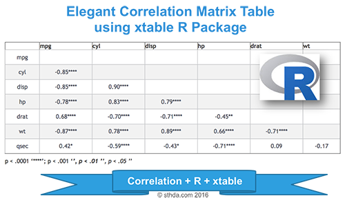
Combine matrix of correlation coefficients and significance levels
Custom function corstars() is used to combine the correlation coefficients and the level of significance. The R code of the function is provided at the end of this article. It requires 2 packages :
- The Hmisc R package to compute the matrix of correlation coefficients and the corresponding p-values.
- The xtable R package for displaying in HTML or Latex format.
Before continuing with the following exercises, you should first copy and paste the source code the function corstars(), which you can find at the bottom of this article.
corstars(mtcars[,1:7], result="html")| mpg | cyl | disp | hp | drat | wt | |
|---|---|---|---|---|---|---|
| mpg | ||||||
| cyl | -0.85**** | |||||
| disp | -0.85**** | 0.90**** | ||||
| hp | -0.78**** | 0.83**** | 0.79**** | |||
| drat | 0.68**** | -0.70**** | -0.71**** | -0.45** | ||
| wt | -0.87**** | 0.78**** | 0.89**** | 0.66**** | -0.71**** | |
| qsec | 0.42* | -0.59*** | -0.43* | -0.71**** | 0.09 | -0.17 |
p < .0001 ‘****’; p < .001 ‘***’, p < .01 ‘**’, p < .05 ‘*’
The code of corstars function (The code is adapted from the one posted on this forum and on this blog ):
# x is a matrix containing the data
# method : correlation method. "pearson"" or "spearman"" is supported
# removeTriangle : remove upper or lower triangle
# results :  if "html" or "latex"
  # the results will be displayed in html or latex format
corstars <-function(x, method=c("pearson", "spearman"), removeTriangle=c("upper", "lower"),
                     result=c("none", "html", "latex")){
    #Compute correlation matrix
    require(Hmisc)
    x <- as.matrix(x)
    correlation_matrix<-rcorr(x, type=method[1])
    R <- correlation_matrix$r # Matrix of correlation coeficients
    p <- correlation_matrix$P # Matrix of p-value

    ## Define notions for significance levels; spacing is important.
    mystars <- ifelse(p < .0001, "****", ifelse(p < .001, "*** ", ifelse(p < .01, "**  ", ifelse(p < .05, "*   ", "    "))))

    ## trunctuate the correlation matrix to two decimal
    R <- format(round(cbind(rep(-1.11, ncol(x)), R), 2))[,-1]

    ## build a new matrix that includes the correlations with their apropriate stars
    Rnew <- matrix(paste(R, mystars, sep=""), ncol=ncol(x))
    diag(Rnew) <- paste(diag(R), " ", sep="")
    rownames(Rnew) <- colnames(x)
    colnames(Rnew) <- paste(colnames(x), "", sep="")

    ## remove upper triangle of correlation matrix
    if(removeTriangle[1]=="upper"){
      Rnew <- as.matrix(Rnew)
      Rnew[upper.tri(Rnew, diag = TRUE)] <- ""
      Rnew <- as.data.frame(Rnew)
    }

    ## remove lower triangle of correlation matrix
    else if(removeTriangle[1]=="lower"){
      Rnew <- as.matrix(Rnew)
      Rnew[lower.tri(Rnew, diag = TRUE)] <- ""
      Rnew <- as.data.frame(Rnew)
    }

    ## remove last column and return the correlation matrix
    Rnew <- cbind(Rnew[1:length(Rnew)-1])
    if (result[1]=="none") return(Rnew)
    else{
      if(result[1]=="html") print(xtable(Rnew), type="html")
      else print(xtable(Rnew), type="latex")
    }
}
Conclusions
- Use cor() function to compute correlation matrix.
- Use lower.tri() and upper.tri() functions to get the lower or upper part of the correlation matrix
- Use xtable R function to display a nice correlation matrix in latex or html format.
Infos
This analysis was performed using R (ver. 3.3.2).Show me some love with the like buttons below... Thank you and please don't forget to share and comment below!!
Montrez-moi un peu d'amour avec les like ci-dessous ... Merci et n'oubliez pas, s'il vous plaît, de partager et de commenter ci-dessous!
Recommended for You!


Recommended for you
This section contains best data science and self-development resources to help you on your path.
Coursera - Online Courses and Specialization
Data science
- Course: Machine Learning: Master the Fundamentals by Standford
- Specialization: Data Science by Johns Hopkins University
- Specialization: Python for Everybody by University of Michigan
- Courses: Build Skills for a Top Job in any Industry by Coursera
- Specialization: Master Machine Learning Fundamentals by University of Washington
- Specialization: Statistics with R by Duke University
- Specialization: Software Development in R by Johns Hopkins University
- Specialization: Genomic Data Science by Johns Hopkins University
Popular Courses Launched in 2020
- Google IT Automation with Python by Google
- AI for Medicine by deeplearning.ai
- Epidemiology in Public Health Practice by Johns Hopkins University
- AWS Fundamentals by Amazon Web Services
Trending Courses
- The Science of Well-Being by Yale University
- Google IT Support Professional by Google
- Python for Everybody by University of Michigan
- IBM Data Science Professional Certificate by IBM
- Business Foundations by University of Pennsylvania
- Introduction to Psychology by Yale University
- Excel Skills for Business by Macquarie University
- Psychological First Aid by Johns Hopkins University
- Graphic Design by Cal Arts
Books - Data Science
Our Books
- Practical Guide to Cluster Analysis in R by A. Kassambara (Datanovia)
- Practical Guide To Principal Component Methods in R by A. Kassambara (Datanovia)
- Machine Learning Essentials: Practical Guide in R by A. Kassambara (Datanovia)
- R Graphics Essentials for Great Data Visualization by A. Kassambara (Datanovia)
- GGPlot2 Essentials for Great Data Visualization in R by A. Kassambara (Datanovia)
- Network Analysis and Visualization in R by A. Kassambara (Datanovia)
- Practical Statistics in R for Comparing Groups: Numerical Variables by A. Kassambara (Datanovia)
- Inter-Rater Reliability Essentials: Practical Guide in R by A. Kassambara (Datanovia)
Others
- R for Data Science: Import, Tidy, Transform, Visualize, and Model Data by Hadley Wickham & Garrett Grolemund
- Hands-On Machine Learning with Scikit-Learn, Keras, and TensorFlow: Concepts, Tools, and Techniques to Build Intelligent Systems by Aurelien Géron
- Practical Statistics for Data Scientists: 50 Essential Concepts by Peter Bruce & Andrew Bruce
- Hands-On Programming with R: Write Your Own Functions And Simulations by Garrett Grolemund & Hadley Wickham
- An Introduction to Statistical Learning: with Applications in R by Gareth James et al.
- Deep Learning with R by François Chollet & J.J. Allaire
- Deep Learning with Python by François Chollet