


Creating and Saving Graphs - R Base Graphs
Previously, we described the essentials of R programming and provided quick start guides for importing data into R.
Pleleminary tasks
Launch RStudio as described here: Running RStudio and setting up your working directory
Prepare your data as described here: Best practices for preparing your data and save it in an external .txt tab or .csv files
Import your data into R as described here: Fast reading of data from txt|csv files into R: readr package.
Here, we’ll use the R built-in mtcars data set.
# Create my_data
my_data <- mtcars
# Print the first 6 rows
head(my_data, 6)
## mpg cyl disp hp drat wt qsec vs am gear carb
## Mazda RX4 21.0 6 160 110 3.90 2.620 16.46 0 1 4 4
## Mazda RX4 Wag 21.0 6 160 110 3.90 2.875 17.02 0 1 4 4
## Datsun 710 22.8 4 108 93 3.85 2.320 18.61 1 1 4 1
## Hornet 4 Drive 21.4 6 258 110 3.08 3.215 19.44 1 0 3 1
## Hornet Sportabout 18.7 8 360 175 3.15 3.440 17.02 0 0 3 2
## Valiant 18.1 6 225 105 2.76 3.460 20.22 1 0 3 1Creating graphs
The R base function plot() can be used to create graphs.
plot(x = my_data$wt, y = my_data$mpg,
     pch = 16, frame = FALSE,
     xlab = "wt", ylab = "mpg", col = "#2E9FDF")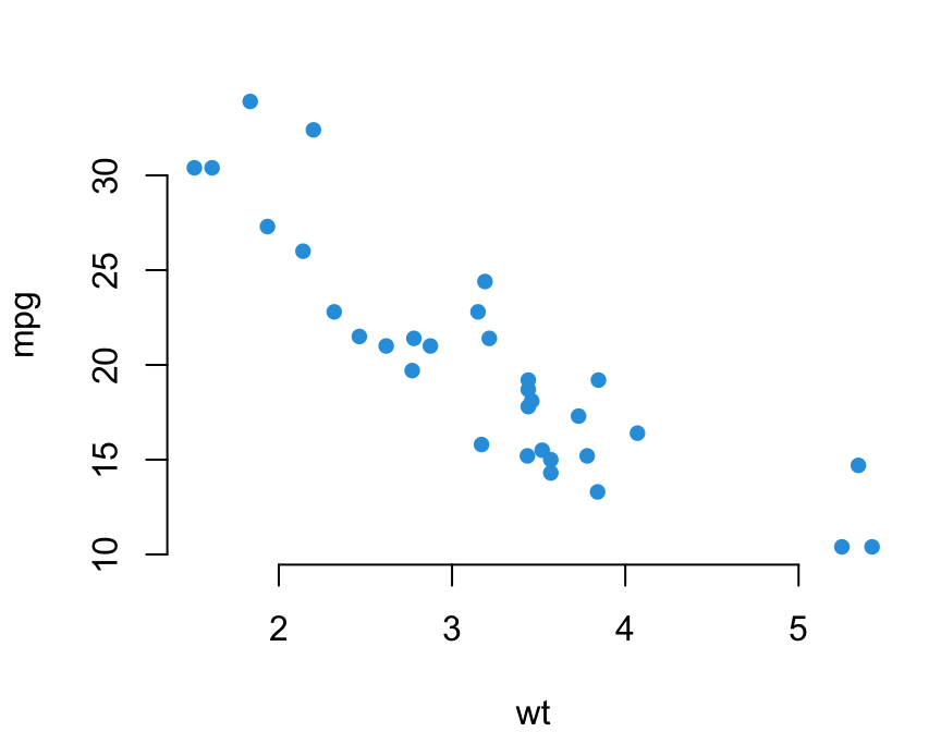
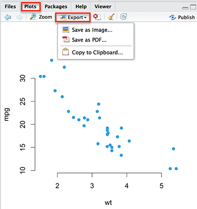
Saving graphs
If you are working with RStudio, the plot can be exported from menu in plot panel (lower right-pannel).
Plots panel –> Export –> Save as Image or Save as PDF
It’s also possible to save the graph using R codes as follow:
- Specify files to save your image using a function such as jpeg(), png(), svg() or pdf(). Additional argument indicating the width and the height of the image can be also used.
- Create the plot
- Close the file with dev.off()
Example:
# Open a pdf file
pdf("rplot.pdf")
# 2. Create a plot
plot(x = my_data$wt, y = my_data$mpg,
     pch = 16, frame = FALSE,
     xlab = "wt", ylab = "mpg", col = "#2E9FDF")
# Close the pdf file
dev.off()
Or use this:
# 1. Open jpeg file
jpeg("rplot.jpg", width = 350, height = "350")
# 2. Create the plot
plot(x = my_data$wt, y = my_data$mpg,
     pch = 16, frame = FALSE,
     xlab = "wt", ylab = "mpg", col = "#2E9FDF")
# 3. Close the file
dev.off()
The R code above, saves the file in the current working directory.
File formats for exporting plots:
- pdf(“rplot.pdf”): pdf file
- png(“rplot.png”): png file
- jpeg(“rplot.jpg”): jpeg file
- postscript(“rplot.ps”): postscript file
- bmp(“rplot.bmp”): bmp file
- win.metafile(“rplot.wmf”): windows metafile
See also
Infos
This analysis has been performed using R statistical software (ver. 3.2.4).
Show me some love with the like buttons below... Thank you and please don't forget to share and comment below!!
Montrez-moi un peu d'amour avec les like ci-dessous ... Merci et n'oubliez pas, s'il vous plaît, de partager et de commenter ci-dessous!
Recommended for You!


Recommended for you
This section contains best data science and self-development resources to help you on your path.
Coursera - Online Courses and Specialization
Data science
- Course: Machine Learning: Master the Fundamentals by Standford
- Specialization: Data Science by Johns Hopkins University
- Specialization: Python for Everybody by University of Michigan
- Courses: Build Skills for a Top Job in any Industry by Coursera
- Specialization: Master Machine Learning Fundamentals by University of Washington
- Specialization: Statistics with R by Duke University
- Specialization: Software Development in R by Johns Hopkins University
- Specialization: Genomic Data Science by Johns Hopkins University
Popular Courses Launched in 2020
- Google IT Automation with Python by Google
- AI for Medicine by deeplearning.ai
- Epidemiology in Public Health Practice by Johns Hopkins University
- AWS Fundamentals by Amazon Web Services
Trending Courses
- The Science of Well-Being by Yale University
- Google IT Support Professional by Google
- Python for Everybody by University of Michigan
- IBM Data Science Professional Certificate by IBM
- Business Foundations by University of Pennsylvania
- Introduction to Psychology by Yale University
- Excel Skills for Business by Macquarie University
- Psychological First Aid by Johns Hopkins University
- Graphic Design by Cal Arts
Books - Data Science
Our Books
- Practical Guide to Cluster Analysis in R by A. Kassambara (Datanovia)
- Practical Guide To Principal Component Methods in R by A. Kassambara (Datanovia)
- Machine Learning Essentials: Practical Guide in R by A. Kassambara (Datanovia)
- R Graphics Essentials for Great Data Visualization by A. Kassambara (Datanovia)
- GGPlot2 Essentials for Great Data Visualization in R by A. Kassambara (Datanovia)
- Network Analysis and Visualization in R by A. Kassambara (Datanovia)
- Practical Statistics in R for Comparing Groups: Numerical Variables by A. Kassambara (Datanovia)
- Inter-Rater Reliability Essentials: Practical Guide in R by A. Kassambara (Datanovia)
Others
- R for Data Science: Import, Tidy, Transform, Visualize, and Model Data by Hadley Wickham & Garrett Grolemund
- Hands-On Machine Learning with Scikit-Learn, Keras, and TensorFlow: Concepts, Tools, and Techniques to Build Intelligent Systems by Aurelien Géron
- Practical Statistics for Data Scientists: 50 Essential Concepts by Peter Bruce & Andrew Bruce
- Hands-On Programming with R: Write Your Own Functions And Simulations by Garrett Grolemund & Hadley Wickham
- An Introduction to Statistical Learning: with Applications in R by Gareth James et al.
- Deep Learning with R by François Chollet & J.J. Allaire
- Deep Learning with Python by François Chollet