Articles - Classification Methods Essentials

Linearity assumption

Here, we’ll check the linear relationship between continuous predictor variables and the logit of the outcome. This can be done by visually inspecting the scatter plot between each predictor and the logit values.

1. Remove qualitative variables from the original data frame and bind the logit values to the data:

# Select only numeric predictors
mydata <- PimaIndiansDiabetes2 %>%
  dplyr::select_if(is.numeric) 
predictors <- colnames(mydata)
# Bind the logit and tidying the data for plot
mydata <- mydata %>%
  mutate(logit = log(probabilities/(1-probabilities))) %>%
  gather(key = "predictors", value = "predictor.value", -logit)

2. Create the scatter plots:

ggplot(mydata, aes(logit, predictor.value))+
  geom_point(size = 0.5, alpha = 0.5) +
  geom_smooth(method = "loess") + 
  theme_bw() + 
  facet_wrap(~predictors, scales = "free_y")

The smoothed scatter plots show that variables glucose, mass, pregnant, pressure and triceps are all quite linearly associated with the diabetes outcome in logit scale.

The variable age and pedigree is not linear and might need some transformations. If the scatter plot shows non-linearity, you need other methods to build the model such as including 2 or 3-power terms, fractional polynomials and spline function (Chapter @ref(polynomial-and-spline-regression)).

Influential values

Influential values are extreme individual data points that can alter the quality of the logistic regression model.

The most extreme values in the data can be examined by visualizing the Cook’s distance values. Here we label the top 3 largest values:

plot(model, which = 4, id.n = 3)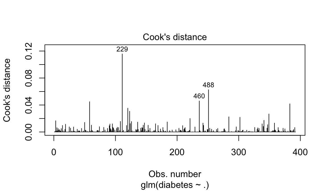

Note that, not all outliers are influential observations. To check whether the data contains potential influential observations, the standardized residual error can be inspected. Data points with an absolute standardized residuals above 3 represent possible outliers and may deserve closer attention.

The following R code computes the standardized residuals (.std.resid) and the Cook’s distance (.cooksd) using the R function augment() [broom package].

# Extract model results
model.data <- augment(model) %>% 
  mutate(index = 1:n()) 

The data for the top 3 largest values, according to the Cook’s distance, can be displayed as follow:

model.data %>% top_n(3, .cooksd)

Plot the standardized residuals:

ggplot(model.data, aes(index, .std.resid)) + 
  geom_point(aes(color = diabetes), alpha = .5) +
  theme_bw()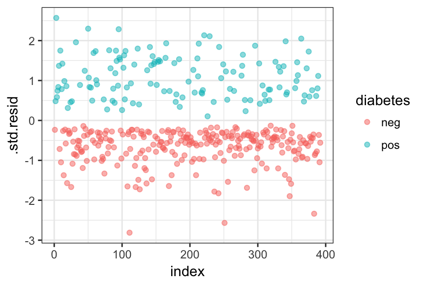

Filter potential influential data points with abs(.std.res) > 3:

model.data %>% 
  filter(abs(.std.resid) > 3)

When you have outliers in a continuous predictor, potential solutions include:

• Removing the concerned records
• Transform the data into log scale
• Use non parametric methods

Multicollinearity

Multicollinearity corresponds to a situation where the data contain highly correlated predictor variables. Read more in Chapter @ref(multicollinearity).

Multicollinearity is an important issue in regression analysis and should be fixed by removing the concerned variables. It can be assessed using the R function vif() [car package], which computes the variance inflation factors:

car::vif(model)

## pregnant  glucose pressure  triceps  insulin     mass pedigree      age 
##     1.89     1.38     1.19     1.64     1.38     1.83     1.03     1.97

As a rule of thumb, a VIF value that exceeds 5 or 10 indicates a problematic amount of collinearity. In our example, there is no collinearity: all variables have a value of VIF well below 5.