T test

Probably one of the most popular research questions is whether two independent samples differ from each other. Student’s t test is one of the common statistical test used for comparing the means of two independent or paired samples.

t test formula is described in detail here and it can be easily computed using t.test() R function. However, one important question is :

Is it always correct to compare means ?

The answer is no, of course. This is explained in the next section

The purpose of this article is :

• Firstly to discuss about why we cannot always use t test
• Secondly to provide an easy to use R function (rquery.t.test()) that will guide the user step by step in order to perform t test satisfying the appropriate conditions.

T test assumptions : Normality and equal variances

Statistical errors are common in scientific literature, and about 50% of the published articles have at least one error. Many of the statistical procedures including correlation, regression, t test, and analysis of variance assume that the data are normally distributed.

These tests are called parametric tests, because their validity depends on the distribution of the data.

A frequent error is to use statistical tests that assume a normal distribution on data that are actually skewed.

As mentioned above, we can not always use Student’s t test to compare means. There are different types of t-test : one-sample t test, the independent two samples t test and the paired t test.

These different tests can be used only in certain conditions :

These assumptions should be taken seriously to draw reliable conclusions.

The outcome of these preliminary test then determines which method should be used for assessing the main hypothesis. Unfortunately, these pretests are not performed automatically by the built-in t.test() R function. This is the reason why, I wrote the rquery.t.test() function which checks first all the t test assumptions and then decides which method to use (parametric or non-parametric) based on the result of the preliminary test.

How to test the normality of data?

With large enough sample sizes (n > 30) the violation of the normality assumption should not cause major problems. This implies that we can ignore the distribution of the data and use parametric tests if we are dealing with large sample sizes.

The central limit theorem tells us that no matter what distribution things have, the sampling distribution tends to be normal if the sample is large enough (n > 30).

However, to be consistent, normality can be checked by visual inspection [normal plots (histogram), Q-Q plot (quantile-quantile plot)] or by significance tests.

• The histogram plot (frequency distribution) provides a visual judgment about whether the distribution is bell shaped.
• The significance test compares the sample distribution to a normal one in order to ascertain whether data show or not a serious deviation from normality.

There are several methods for normality test such as Kolmogorov-Smirnov (K-S) normality test and Shapiro-Wilk’s test.

The null hypothesis of these tests is that “sample distribution is normal”. If the test is significant, the distribution is non-normal.

Shapiro-Wilk’s method is widely recommended for normality test and it provides better power than K-S. It is based on the correlation between the data and the corresponding normal scores.

Note that, normality test is sensitive to sample size. Small samples most often pass normality tests. Therefore, it’s important to combine visual inspection and significance test in order to take the right decision.

Question : To test or not to test normality ?

Normality test and the others assumptions made by parametric tests should be pretested before continuing with the main test. For example, in medical research, normally distributed data are the exception rather than the rule. In such situations, the use of parametric methods is discouraged, and non-parametric tests (which are also referred to as distribution-free tests) such as the two-samples Wilcoxon test are recommended instead.

In rquery.t.test() function, Shapiro-Wilk’s normality test is used and, histogram and Q-Q plots are automatically displayed for visual inspection.

How to test the equality of variances ?

The standard two independent samples t test assumes also that the samples have equal variances. If the two samples, being compared, follow normal distribution, F test can be performed to compare the variances.

The null hypothesis of F test is that the variances of the two populations are equal. If the test is significant, null hypothesis are rejected and then we can conclude that the variances are significantly different.

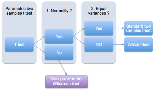
What to do when the conditions are not met for t test ?

If the two samples are normally distributed, but with unequal variances, the Welch t test can be used (figure below). Welch t-test is an adaptation of Student’s t test used when the equality of variances of the two samples cannot be assumed.

rquery.t.test : smart t.test function

As mentioned above, this function is an improvement of the built-in t.test() R function. It can be used to perform one or two sample t-tests (paired and unpaired). Its advantage over the basic t.test() function is that : it checks automatically the distribution of the data and the equality of the two sample variances (in the case of independent t test).

Before calculating t-test, the rquery.t.test function performs the following steps :

1. First, The Shapiro-Wilk test is used to perform normality test. If the samples are not normally distributed, the rquery.t.test function will warn and suggest you to do a wilcoxon test.

2. An F test comparing the variances of the two samples is used to check the assumption of homogeneity of variances (in the case of independent t test) :

• If the two variances are assumed equal : The classic Student’s t-test is performed
• If the two variances are significantly different: the Welch t-test is automatically applied.

Note that the R code of rquery.t.test() function is provided at the end of this document.

A simplified format of the function is :

rquery.t.test(x, y = NULL, paired = FALSE, graph = TRUE, ...)

One sample t-test : Compare an observed mean with a theoretical mean

source('http://www.sthda.com/upload/rquery_t_test.r')
set.seed(123456789)
x<-rnorm(100) # generate some data
rquery.t.test(x, mu=0)

    One Sample t-test
data:  x
t = 0.2606, df = 99, p-value = 0.7949
alternative hypothesis: true mean is not equal to 0
95 percent confidence interval:
 -0.1657  0.2159
sample estimates:
mean of x 
  0.02506 

Read more by following this link : one sample t test

Independent t-test : Compare the means of two unpaired samples

Case 1 - The two groups of samples are normally distributed and have equal variances:

source('http://www.sthda.com/upload/rquery_t_test.r')
set.seed(123456789)
x<-rnorm(100, mean=2, sd=0.9)
y<-rnorm(100, mean=4, sd=1)
rquery.t.test(x, y)

    Two Sample t-test
data:  x and y
t = -16.85, df = 198, p-value < 2.2e-16
alternative hypothesis: true difference in means is not equal to 0
95 percent confidence interval:
 -2.449 -1.935
sample estimates:
mean of x mean of y 
    2.023     4.215 

The classic two samples t-test is automatically used.

Case 2 - The two samples are normally distributed but the variances are unequal:

source('http://www.sthda.com/upload/rquery_t_test.r')
set.seed(123456789)
x<-rnorm(100, mean=2, sd=0.9)
y<-rnorm(100, mean=2, sd=3)
rquery.t.test(x, y)

    Welch Two Sample t-test
data:  x and y
t = -2.043, df = 116.3, p-value = 0.04326
alternative hypothesis: true difference in means is not equal to 0
95 percent confidence interval:
 -1.22327 -0.01913
sample estimates:
mean of x mean of y 
    2.023     2.644 

The Weltch t-test is automatically used.

Case 3 - The samples are not normally distributed:

source('http://www.sthda.com/upload/rquery_t_test.r')
set.seed(123456789)
x<-rnorm(100, mean=2, sd=0.9)
x<-c(x, 10,20) # add some outliers
y<-rnorm(100, mean=4, sd=1)
rquery.t.test(x, y)

Warning: x or y is not normally distributed : Shapiro test p-value : 2e-17 (for x) and 0.5 (for y).
 Use a non parametric test like Wilcoxon test.

    Welch Two Sample t-test
data:  x and y
t = -8.374, df = 142.2, p-value = 4.809e-14
alternative hypothesis: true difference in means is not equal to 0
95 percent confidence interval:
 -2.395 -1.480
sample estimates:
mean of x mean of y 
    2.277     4.215 

A warning message is automatically displayed and the rquery.t.test function will suggest you to perform a non-parametric test like wilcoxon test.

Paired t test : Compare two dependent samples

source('http://www.sthda.com/upload/rquery_t_test.r')
set.seed(123456789)
x<-rnorm(30, mean=10, sd=2)
y<-rnorm(30, mean=50, sd=3)
rquery.t.test(x, y, paired=TRUE)

    Paired t-test
data:  x and y
t = -56.5, df = 29, p-value < 2.2e-16
alternative hypothesis: true difference in means is not equal to 0
95 percent confidence interval:
 -41.63 -38.72
sample estimates:
mean of the differences 
                 -40.17 

Read more on paired t test

Online t-test calculator

The R code of rquery.t.test function

#++++++++++++++++++++++++
# rquery.t.test
#+++++++++++++++++++++++
# Description : Performs one or two samples t-test
# x : a (non-empty) numeric vector of data values.
# y : an optional (non-empty) numeric vector of data values
# paired : if TRUE, paired t-test is performed
# graph : if TRUE, the distribution of the data is shown
  # for the inspection of normality
# ... : further arguments to be passed to the built-in t.test() R function
# 1. shapiro.test is used to check normality
# 2. F-test is performed to check equality of variances
# If the variances are different, then Welch t-test is used
rquery.t.test<-function(x, y = NULL, paired = FALSE, graph = TRUE, ...)
{
  # I. Preliminary test : normality and variance tests
  # ~~~~~~~~~~~~~~~~~~~~~~~~~~~~~~~~~~~~~~~~~~~~~~
  var.equal = FALSE # by default
  
  # I.1 One sample t test
  if(is.null(y)){
    if(graph) par(mfrow=c(1,2))
    shapiro.px<-normaTest(x, graph, 
                          hist.title="X - Histogram",
                          qq.title="X - Normal Q-Q Plot")
    if(shapiro.px < 0.05)
      warning("x is not normally distributed :",
              " Shapiro-Wilk test p-value : ", shapiro.px, 
              ".\n Use a non-parametric test like Wilcoxon test.")
  }
  
  # I.2 Two samples t test
  if(!is.null(y)){
    
      # I.2.a unpaired t test
      if(!paired){
          if(graph) par(mfrow=c(2,2))
          # normality test
          shapiro.px<-normaTest(x, graph, 
                                hist.title="X - Histogram",
                                qq.title="X - Normal Q-Q Plot")
          shapiro.py<-normaTest(y, graph,
                                hist.title="Y - Histogram",
                                qq.title="Y - Normal Q-Q Plot")
          if(shapiro.px < 0.05 | shapiro.py < 0.05){
              warning("x or y is not normally distributed :",
                      " Shapiro test p-value : ", shapiro.px,
                      " (for x) and ", shapiro.py, " (for y)",
                      ".\n Use a non parametric test like Wilcoxon test.")
            }
          # Check for equality of variances
          if(var.test(x,y)$p.value >= 0.05) var.equal=TRUE
        } 
      
      # I.2.b Paired t-test
      else {
        if(graph) par(mfrow=c(1,2))
        d = x-y 
        shapiro.pd<-normaTest(d, graph, 
                              hist.title="D - Histogram",
                              qq.title="D - Normal Q-Q Plot")
        if(shapiro.pd < 0.05 )
          warning("The difference d ( = x-y) is not normally distributed :",
                  " Shapiro-Wilk test p-value : ", shapiro.pd, 
                  ".\n Use a non-parametric test like Wilcoxon test.")
      } 
      
   }
  
  # II. Student's t-test
  # ~~~~~~~~~~~~~~~~~~~~~~~~~~~~
  res <- t.test(x, y, paired=paired, var.equal=var.equal, ...)
  return(res)
}
#+++++++++++++++++++++++
# Helper function
#+++++++++++++++++++++++
# Performs normality test using Shapiro Wilk's method
# The histogram and Q-Q plot of the data are plotted
# x : a (non-empty) numeric vector of data values.
# graph : possible values are TRUE or FALSE. If TRUE,
  # the histogram and the Q-Q plot of the data are displayed
# hist.title : title of the histogram
# qq.title : title of the Q-Q plot
normaTest<-function(x, graph=TRUE, 
                    hist.title="Histogram", 
                    qq.title="Normal Q-Q Plot",...)
  {  
  # Significance test
  #++++++++++++++++++++++
  shapiro.p<-signif(shapiro.test(x)$p.value,1) 
  
  if(graph){
    # Plot : Visual inspection
    #++++++++++++++++
    h<-hist(x, col="lightblue", main=hist.title, 
            xlab="Data values", ...)
    m<-round(mean(x),1)
    s<-round(sd(x),1)
    mtext(paste0("Mean : ", m, "; SD : ", s),
          side=3, cex=0.8)
    # add normal curve
    xfit<-seq(min(x),max(x),length=40)
    yfit<-dnorm(xfit,mean=mean(x),sd=sd(x))
    yfit <- yfit*diff(h$mids[1:2])*length(x)
    lines(xfit, yfit, col="red", lwd=2)
    # qq plot
    qqnorm(x, pch=19, frame.plot=FALSE,main=qq.title)
    qqline(x)
    mtext(paste0("Shapiro-Wilk, p-val : ", shapiro.p),
          side=3, cex=0.8)
  }
  return(shapiro.p)
}

Infos

This analysis has been performed with R (ver. 3.1.0).

References

1. Asghar Ghasemi, Saleh Zahediasl; Normality Tests for Statistical Analysis: A Guide for Non-Statisticians; Int J Endocrinol Metab. 2012;10(2):486-489.
2. Rochon J1, Gondan M, Kieser M.; To test or not to test: Preliminary assessment of normality when comparing two independent samples; BMC Med Res Methodol. 2012 Jun 19;12:81.

Recommended for you