


Principal Component and Partial Least Squares Regression Essentials
This chapter presents regression methods based on dimension reduction techniques, which can be very useful when you have a large data set with multiple correlated predictor variables.
Generally, all dimension reduction methods work by first summarizing the original predictors into few new variables called principal components (PCs), which are then used as predictors to fit the linear regression model. These methods avoid multicollinearity between predictors, which a big issue in regression setting (see Chapter @ref(multicollinearity)).
When using the dimension reduction methods, it’s generally recommended to standardize each predictor to make them comparable. Standardization consists of dividing the predictor by its standard deviation.
Here, we described two well known regression methods based on dimension reduction: Principal Component Regression (PCR) and Partial Least Squares (PLS) regression. We also provide practical examples in R.
Contents:

Principal component regression
The principal component regression (PCR) first applies Principal Component Analysis on the data set to summarize the original predictor variables into few new variables also known as principal components (PCs), which are a linear combination of the original data.
These PCs are then used to build the linear regression model. The number of principal components, to incorporate in the model, is chosen by cross-validation (cv). Note that, PCR is suitable when the data set contains highly correlated predictors.
Partial least squares regression
A possible drawback of PCR is that we have no guarantee that the selected principal components are associated with the outcome. Here, the selection of the principal components to incorporate in the model is not supervised by the outcome variable.
An alternative to PCR is the Partial Least Squares (PLS) regression, which identifies new principal components that not only summarizes the original predictors, but also that are related to the outcome. These components are then used to fit the regression model. So, compared to PCR, PLS uses a dimension reduction strategy that is supervised by the outcome.
Like PCR, PLS is convenient for data with highly-correlated predictors. The number of PCs used in PLS is generally chosen by cross-validation. Predictors and the outcome variables should be generally standardized, to make the variables comparable.
Loading required R packages
tidyversefor easy data manipulation and visualizationcaretfor easy machine learning workflowpls, for computing PCR and PLS
library(tidyverse)
library(caret)
library(pls)
Preparing the data
We’ll use the Boston data set [in MASS package], introduced in Chapter @ref(regression-analysis), for predicting the median house value (mdev), in Boston Suburbs, based on multiple predictor variables.
We’ll randomly split the data into training set (80% for building a predictive model) and test set (20% for evaluating the model). Make sure to set seed for reproducibility.
# Load the data
data("Boston", package = "MASS")
# Split the data into training and test set
set.seed(123)
training.samples <- Boston$medv %>%
  createDataPartition(p = 0.8, list = FALSE)
train.data  <- Boston[training.samples, ]
test.data <- Boston[-training.samples, ]
Computation
The R function train() [caret package] provides an easy workflow to compute PCR and PLS by invoking the pls package. It has an option named method, which can take the value pcr or pls.
An additional argument is scale = TRUE for standardizing the variables to make them comparable.
caret uses cross-validation to automatically identify the optimal number of principal components (ncomp) to be incorporated in the model.
Here, we’ll test 10 different values of the tuning parameter ncomp. This is specified using the option tuneLength. The optimal number of principal components is selected so that the cross-validation error (RMSE) is minimized.
Computing principal component regression
# Build the model on training set
set.seed(123)
model <- train(
  medv~., data = train.data, method = "pcr",
  scale = TRUE,
  trControl = trainControl("cv", number = 10),
  tuneLength = 10
  )
# Plot model RMSE vs different values of components
plot(model)
# Print the best tuning parameter ncomp that
# minimize the cross-validation error, RMSE
model$bestTune
## ncomp
## 5 5# Summarize the final model
summary(model$finalModel)## Data: X dimension: 407 13
## Y dimension: 407 1
## Fit method: svdpc
## Number of components considered: 5
## TRAINING: % variance explained
## 1 comps 2 comps 3 comps 4 comps 5 comps
## X 47.48 58.40 68.00 74.75 80.94
## .outcome 38.10 51.02 64.43 65.24 71.17# Make predictions
predictions <- model %>% predict(test.data)
# Model performance metrics
data.frame(
RMSE = caret::RMSE(predictions, test.data$medv),
Rsquare = caret::R2(predictions, test.data$medv)
)## RMSE Rsquare
## 1 5.18 0.645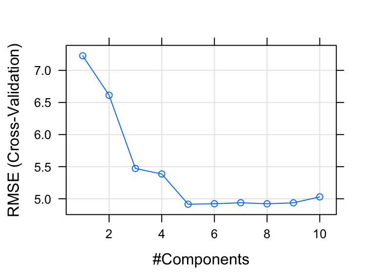
The plot shows the prediction error (RMSE, Chapter @ref(regression-model-accuracy-metrics)) made by the model according to the number of principal components incorporated in the model.
Our analysis shows that, choosing five principal components (ncomp = 5) gives the smallest prediction error RMSE.
The summary() function also provides the percentage of variance explained in the predictors (x) and in the outcome (medv) using different numbers of components.
For example, 80.94% of the variation (or information) contained in the predictors are captured by 5 principal components (ncomp = 5). Additionally, setting ncomp = 5, captures 71% of the information in the outcome variable (medv), which is good.
Taken together, cross-validation identifies ncomp = 5 as the optimal number of PCs that minimize the prediction error (RMSE) and explains enough variation in the predictors and in the outcome.
Computing partial least squares
The R code is just like that of the PCR method.
# Build the model on training set
set.seed(123)
model <- train(
  medv~., data = train.data, method = "pls",
  scale = TRUE,
  trControl = trainControl("cv", number = 10),
  tuneLength = 10
  )
# Plot model RMSE vs different values of components
plot(model)
# Print the best tuning parameter ncomp that
# minimize the cross-validation error, RMSE
model$bestTune
## ncomp
## 9 9# Summarize the final model
summary(model$finalModel)## Data: X dimension: 407 13
## Y dimension: 407 1
## Fit method: oscorespls
## Number of components considered: 9
## TRAINING: % variance explained
## 1 comps 2 comps 3 comps 4 comps 5 comps 6 comps 7 comps
## X 46.19 57.32 64.15 69.76 75.63 78.66 82.85
## .outcome 50.90 71.84 73.71 74.71 75.18 75.35 75.42
## 8 comps 9 comps
## X 85.92 90.36
## .outcome 75.48 75.49# Make predictions
predictions <- model %>% predict(test.data)
# Model performance metrics
data.frame(
RMSE = caret::RMSE(predictions, test.data$medv),
Rsquare = caret::R2(predictions, test.data$medv)
)## RMSE Rsquare
## 1 4.99 0.671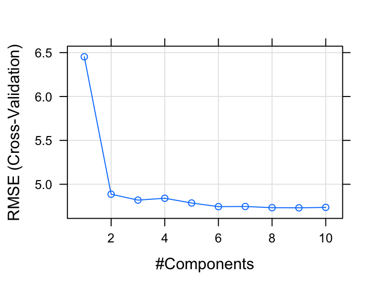
The optimal number of principal components included in the PLS model is 9. This captures 90% of the variation in the predictors and 75% of the variation in the outcome variable (medv).
In our example, the cross-validation error RMSE obtained with the PLS model is lower than the RMSE obtained using the PCR method. So, the PLS model is the best model, for explaining our data, compared to the PCR model.
Discussion
This chapter describes principal component based regression methods, including principal component regression (PCR) and partial least squares regression (PLS). These methods are very useful for multivariate data containing correlated predictors.
The presence of correlation in the data allows to summarize the data into few non-redundant components that can be used in the regression model.
Compared to ridge regression and lasso (Chapter @ref(penalized-regression)), the final PCR and PLS models are more difficult to interpret, because they do not perform any kind of variable selection or even directly produce regression coefficient estimates.