Articles - Classification Methods Essentials

Logistic function

The standard logistic regression function, for predicting the outcome of an observation given a predictor variable (x), is an s-shaped curve defined as p = exp(y) / [1 + exp(y)] (James et al. 2014). This can be also simply written as p = 1/[1 + exp(-y)], where:

• y = b0 + b1*x,
• exp() is the exponential and
• p is the probability of event to occur (1) given x. Mathematically, this is written as p(event=1|x) and abbreviated asp(x), sopx = 1/[1 + exp(-(b0 + b1*x))]`

By a bit of manipulation, it can be demonstrated that p/(1-p) = exp(b0 + b1*x). By taking the logarithm of both sides, the formula becomes a linear combination of predictors: log[p/(1-p)] = b0 + b1*x.

When you have multiple predictor variables, the logistic function looks like: log[p/(1-p)] = b0 + b1*x1 + b2*x2 + ... + bn*xn

b0 and b1 are the regression beta coefficients. A positive b1 indicates that increasing x will be associated with increasing p. Conversely, a negative b1 indicates that increasing x will be associated with decreasing p.

The quantity log[p/(1-p)] is called the logarithm of the odd, also known as log-odd or logit.

The odds reflect the likelihood that the event will occur. It can be seen as the ratio of “successes” to “non-successes”. Technically, odds are the probability of an event divided by the probability that the event will not take place (P. Bruce and Bruce 2017). For example, if the probability of being diabetes-positive is 0.5, the probability of “won’t be” is 1-0.5 = 0.5, and the odds are 1.0.

Note that, the probability can be calculated from the odds as p = Odds/(1 + Odds).

Loading required R packages

• tidyverse for easy data manipulation and visualization
• caret for easy machine learning workflow

library(tidyverse)
library(caret)
theme_set(theme_bw())

Preparing the data

Logistic regression works for a data that contain continuous and/or categorical predictor variables.

Performing the following steps might improve the accuracy of your model

• Remove potential outliers
• Make sure that the predictor variables are normally distributed. If not, you can use log, root, Box-Cox transformation.
• Remove highly correlated predictors to minimize overfitting. The presence of highly correlated predictors might lead to an unstable model solution.

Here, we’ll use the PimaIndiansDiabetes2 [in mlbench package], introduced in Chapter @ref(classification-in-r), for predicting the probability of being diabetes positive based on multiple clinical variables.

We’ll randomly split the data into training set (80% for building a predictive model) and test set (20% for evaluating the model). Make sure to set seed for reproducibility.

# Load the data and remove NAs
data("PimaIndiansDiabetes2", package = "mlbench")
PimaIndiansDiabetes2 <- na.omit(PimaIndiansDiabetes2)
# Inspect the data
sample_n(PimaIndiansDiabetes2, 3)
# Split the data into training and test set
set.seed(123)
training.samples <- PimaIndiansDiabetes2$diabetes %>% 
  createDataPartition(p = 0.8, list = FALSE)
train.data  <- PimaIndiansDiabetes2[training.samples, ]
test.data <- PimaIndiansDiabetes2[-training.samples, ]

Computing logistic regression

The R function glm(), for generalized linear model, can be used to compute logistic regression. You need to specify the option family = binomial, which tells to R that we want to fit logistic regression.

# Fit the model
model <- glm( diabetes ~., data = train.data, family = binomial)
# Summarize the model
summary(model)
# Make predictions
probabilities <- model %>% predict(test.data, type = "response")
predicted.classes <- ifelse(probabilities > 0.5, "pos", "neg")
# Model accuracy
mean(predicted.classes == test.data$diabetes)

model <- glm( diabetes ~ glucose, data = train.data, family = binomial)
summary(model)$coef

##             Estimate Std. Error z value Pr(>|z|)
## (Intercept)  -6.3267     0.7241   -8.74 2.39e-18
## glucose       0.0437     0.0054    8.09 6.01e-16

newdata <- data.frame(glucose = c(20,  180))
probabilities <- model %>% predict(newdata, type = "response")
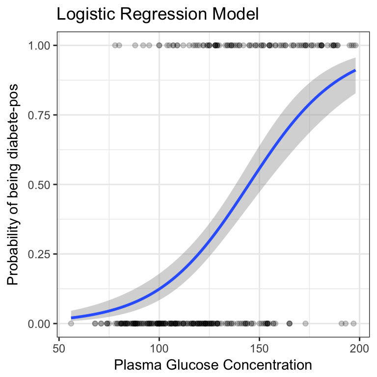
predicted.classes <- ifelse(probabilities > 0.5, "pos", "neg")
predicted.classes

train.data %>%
  mutate(prob = ifelse(diabetes == "pos", 1, 0)) %>%
  ggplot(aes(glucose, prob)) +
  geom_point(alpha = 0.2) +
  geom_smooth(method = "glm", method.args = list(family = "binomial")) +
  labs(
    title = "Logistic Regression Model", 
    x = "Plasma Glucose Concentration",
    y = "Probability of being diabete-pos"
    )

model <- glm( diabetes ~ glucose + mass + pregnant, 
                data = train.data, family = binomial)
summary(model)$coef

model <- glm( diabetes ~., data = train.data, family = binomial)
summary(model)$coef

##             Estimate Std. Error z value Pr(>|z|)
## (Intercept) -9.50372    1.31719  -7.215 5.39e-13
## pregnant     0.04571    0.06218   0.735 4.62e-01
## glucose      0.04230    0.00657   6.439 1.20e-10
## pressure    -0.00700    0.01291  -0.542 5.87e-01
## triceps      0.01858    0.01861   0.998 3.18e-01
## insulin     -0.00159    0.00139  -1.144 2.52e-01
## mass         0.04502    0.02887   1.559 1.19e-01
## pedigree     0.96845    0.46020   2.104 3.53e-02
## age          0.04256    0.02158   1.972 4.86e-02

coef(model)
summary(model )$coef

Interpretation

It can be seen that only 5 out of the 8 predictors are significantly associated to the outcome. These include: pregnant, glucose, pressure, mass and pedigree.

The coefficient estimate of the variable glucose is b = 0.045, which is positive. This means that an increase in glucose is associated with increase in the probability of being diabetes-positive. However the coefficient for the variable pressure is b = -0.007, which is negative. This means that an increase in blood pressure will be associated with a decreased probability of being diabetes-positive.

An important concept to understand, for interpreting the logistic beta coefficients, is the odds ratio. An odds ratio measures the association between a predictor variable (x) and the outcome variable (y). It represents the ratio of the odds that an event will occur (event = 1) given the presence of the predictor x (x = 1), compared to the odds of the event occurring in the absence of that predictor (x = 0).

For a given predictor (say x1), the associated beta coefficient (b1) in the logistic regression function corresponds to the log of the odds ratio for that predictor.

If the odds ratio is 2, then the odds that the event occurs (event = 1) are two times higher when the predictor x is present (x = 1) versus x is absent (x = 0).

For example, the regression coefficient for glucose is 0.042. This indicate that one unit increase in the glucose concentration will increase the odds of being diabetes-positive by exp(0.042) 1.04 times.

From the logistic regression results, it can be noticed that some variables - triceps, insulin and age - are not statistically significant. Keeping them in the model may contribute to overfitting. Therefore, they should be eliminated. This can be done automatically using statistical techniques, including stepwise regression and penalized regression methods. This methods are described in the next section. Briefly, they consist of selecting an optimal model with a reduced set of variables, without compromising the model curacy.

Here, as we have a small number of predictors (n = 9), we can select manually the most significant:

model <- glm( diabetes ~ pregnant + glucose + pressure + mass + pedigree, 
                data = train.data, family = binomial)

Making predictions

We’ll make predictions using the test data in order to evaluate the performance of our logistic regression model.

The procedure is as follow:

1. Predict the class membership probabilities of observations based on predictor variables
2. Assign the observations to the class with highest probability score (i.e above 0.5)

The R function predict() can be used to predict the probability of being diabetes-positive, given the predictor values.

Predict the probabilities of being diabetes-positive:

probabilities <- model %>% predict(test.data, type = "response")
head(probabilities)

##     21     25     28     29     32     36 
## 0.3914 0.6706 0.0501 0.5735 0.6444 0.1494

Which classes do these probabilities refer to? In our example, the output is the probability that the diabetes test will be positive. We know that these values correspond to the probability of the test to be positive, rather than negative, because the contrasts() function indicates that R has created a dummy variable with a 1 for “pos” and “0” for neg. The probabilities always refer to the class dummy-coded as “1”.

Check the dummy coding:

contrasts(test.data$diabetes)

##     pos
## neg   0
## pos   1

Predict the class of individuals:

The following R code categorizes individuals into two groups based on their predicted probabilities (p) of being diabetes-positive. Individuals, with p above 0.5 (random guessing), are considered as diabetes-positive.

predicted.classes <- ifelse(probabilities > 0.5, "pos", "neg")
head(predicted.classes)

##    21    25    28    29    32    36 
## "neg" "pos" "neg" "pos" "pos" "neg"

Assessing model accuracy

The model accuracy is measured as the proportion of observations that have been correctly classified. Inversely, the classification error is defined as the proportion of observations that have been misclassified.

Proportion of correctly classified observations:

mean(predicted.classes == test.data$diabetes)

## [1] 0.756

Note that, there are several metrics for evaluating the performance of a classification model (Chapter @ref(classification-model-evaluation)).

Discussion

In this chapter, we have described how logistic regression works and we have provided R codes to compute logistic regression. Additionally, we demonstrated how to make predictions and to assess the model accuracy. Logistic regression model output is very easy to interpret compared to other classification methods. Additionally, because of its simplicity it is less prone to overfitting than flexible methods such as decision trees.

Note that, many concepts for linear regression hold true for the logistic regression modeling. For example, you need to perform some diagnostics (Chapter @ref(logistic-regression-assumptions-and-diagnostics)) to make sure that the assumptions made by the model are met for your data.

Furthermore, you need to measure how good the model is in predicting the outcome of new test data observations. Here, we described how to compute the raw classification accuracy, but not that other important performance metric exists (Chapter @ref(classification-model-evaluation))

In a situation, where you have many predictors you can select, without compromising the prediction accuracy, a minimal list of predictor variables that contribute the most to the model using stepwise regression (Chapter @ref(stepwise-logistic-regression)) and lasso regression techniques (Chapter @ref(penalized-logistic-regression)).

Additionally, you can add interaction terms in the model, or include spline terms.

The same problems concerning confounding and correlated variables apply to logistic regression (see Chapter @ref(confounding-variables) and @ref(multicollinearity)).

You can also fit generalized additive models (Chapter @ref(polynomial-and-spline-regression)), when linearity of the predictor cannot be assumed. This can be done using the mgcv package:

library("mgcv")
# Fit the model
gam.model <- gam(diabetes ~ s(glucose) + mass + pregnant,
                 data = train.data, family = "binomial")
# Summarize model
summary(gam.model )
# Make predictions
probabilities <- gam.model %>% predict(test.data, type = "response")
predicted.classes <- ifelse(probabilities> 0.5, "pos", "neg")
# Model Accuracy
mean(predicted.classes == test.data$diabetes)

Logistic regression is limited to only two-class classification problems. There is an extension, called multinomial logistic regression, for multiclass classification problem (Chapter @ref(multinomial-logistic-regression)).

Note that, the most popular method, for multiclass tasks, is the Linear Discriminant Analysis (Chapter @ref(discriminant-analysis)).

References

Bruce, Peter, and Andrew Bruce. 2017. Practical Statistics for Data Scientists. O’Reilly Media.
James, Gareth, Daniela Witten, Trevor Hastie, and Robert Tibshirani. 2014. An Introduction to Statistical Learning: With Applications in R. Springer Publishing Company, Incorporated.