


KNN: K-Nearest Neighbors Essentials
The k-nearest neighbors (KNN) algorithm is a simple machine learning method used for both classification and regression. The kNN algorithm predicts the outcome of a new observation by comparing it to k similar cases in the training data set, where k is defined by the analyst.
In this chapter, we start by describing the basics of the KNN algorithm for both classification and regression settings. Next, we provide practical example in R for preparing the data and computing KNN model.
Additionally, you’ll learn how to make predictions and to assess the performance of the built model in the predicting the outcome of new test observations.
Contents:

KNN algorithm
- KNN algorithm for classification:
To classify a given new observation (new_obs), the k-nearest neighbors method starts by identifying the k most similar training observations (i.e. neighbors) to our new_obs, and then assigns new_obs to the class containing the majority of its neighbors.
- KNN algorithm for regression:
Similarly, to predict a continuous outcome value for given new observation (new_obs), the KNN algorithm computes the average outcome value of the k training observations that are the most similar to new_obs, and returns this value as new_obs predicted outcome value.
- Similarity measures:
Note that, the (dis)similarity between observations is generally determined using Euclidean distance measure, which is very sensitive to the scale on which predictor variable measurements are made. So, it’s generally recommended to standardize (i.e., normalize) the predictor variables for making their scales comparable.
The following sections shows how to build a k-nearest neighbor predictive model for classification and regression settings.
Loading required R packages
tidyversefor easy data manipulation and visualizationcaretfor easy machine learning workflow
library(tidyverse)
library(caret)
Classification
Example of data set
Data set: PimaIndiansDiabetes2 [in mlbench package], introduced in Chapter @ref(classification-in-r), for predicting the probability of being diabetes positive based on multiple clinical variables.
We’ll randomly split the data into training set (80% for building a predictive model) and test set (20% for evaluating the model). Make sure to set seed for reproducibility.
# Load the data and remove NAs
data("PimaIndiansDiabetes2", package = "mlbench")
PimaIndiansDiabetes2 <- na.omit(PimaIndiansDiabetes2)
# Inspect the data
sample_n(PimaIndiansDiabetes2, 3)
# Split the data into training and test set
set.seed(123)
training.samples <- PimaIndiansDiabetes2$diabetes %>%
  createDataPartition(p = 0.8, list = FALSE)
train.data  <- PimaIndiansDiabetes2[training.samples, ]
test.data <- PimaIndiansDiabetes2[-training.samples, ]
Computing KNN classifier
We’ll use the caret package, which automatically tests different possible values of k, then chooses the optimal k that minimizes the cross-validation (“cv”) error, and fits the final best KNN model that explains the best our data.
Additionally caret can automatically preprocess the data in order to normalize the predictor variables.
We’ll use the following arguments in the function train():
trControl, to set up 10-fold cross validationpreProcess, to normalize the datatuneLength, to specify the number of possible k values to evaluate
# Fit the model on the training set
set.seed(123)
model <- train(
  diabetes ~., data = train.data, method = "knn",
  trControl = trainControl("cv", number = 10),
  preProcess = c("center","scale"),
  tuneLength = 20
  )
# Plot model accuracy vs different values of k
plot(model)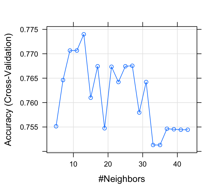
# Print the best tuning parameter k that
# maximizes model accuracy
model$bestTune
## k
## 5 13# Make predictions on the test data
predicted.classes <- model %>% predict(test.data)
head(predicted.classes)## [1] neg pos neg pos pos neg
## Levels: neg pos# Compute model accuracy rate
mean(predicted.classes == test.data$diabetes)## [1] 0.769The overall prediction accuracy of our model is 76.9%, which is good (see Chapter @ref(classification-model-evaluation) for learning key metrics used to evaluate a classification model performance).
KNN for regression
In this section, we’ll describe how to predict a continuous variable using KNN.
We’ll use the Boston data set [in MASS package], introduced in Chapter @ref(regression-analysis), for predicting the median house value (mdev), in Boston Suburbs, using different predictor variables.
- Randomly split the data into training set (80% for building a predictive model) and test set (20% for evaluating the model). Make sure to set seed for reproducibility.
# Load the data
data("Boston", package = "MASS")
# Inspect the data
sample_n(Boston, 3)
# Split the data into training and test set
set.seed(123)
training.samples <- Boston$medv %>%
  createDataPartition(p = 0.8, list = FALSE)
train.data  <- Boston[training.samples, ]
test.data <- Boston[-training.samples, ]- Compute KNN using caret.
The best k is the one that minimize the prediction error RMSE (root mean squared error).
The RMSE corresponds to the square root of the average difference between the observed known outcome values and the predicted values, RMSE = mean((observeds - predicteds)^2) %>% sqrt(). The lower the RMSE, the better the model.
# Fit the model on the training set
set.seed(123)
model <- train(
  medv~., data = train.data, method = "knn",
  trControl = trainControl("cv", number = 10),
  preProcess = c("center","scale"),
  tuneLength = 10
  )
# Plot model error RMSE vs different values of k
plot(model)
# Best tuning parameter k that minimize the RMSE
model$bestTune
# Make predictions on the test data
predictions <- model %>% predict(test.data)
head(predictions)
# Compute the prediction error RMSE
RMSE(predictions, test.data$medv)
Discussion
This chapter describes the basics of KNN (k-nearest neighbors) modeling, which is conceptually, one of the simpler machine learning method.
It’s recommended to standardize the data when performing the KNN analysis. We provided R codes to easily compute KNN predictive model and to assess the model performance on test data.
When fitting the KNN algorithm, the analyst needs to specify the number of neighbors (k) to be considered in the KNN algorithm for predicting the outcome of an observation. The choice of k considerably impacts the output of KNN. k = 1 corresponds to a highly flexible method resulting to a training error rate of 0 (overfitting), but the test error rate may be quite high.
You need to test multiple k-values to decide an optimal value for your data. This can be done automatically using the caret package, which chooses a value of k that minimize the cross-validation error @ref(cross-validation).