Articles - ggpubr: Publication Ready Plots

In this article, we’ll explain how to create histograms/density plots with text labels using the ggpubr package.

I used this type of plots in my recent scientific publication entitled “Global miRNA expression analysis identifies novel key regulators of plasma cell differentiation and malignant plasma cell”, in Nucleic Acids Research Journal, where I was interested to visualize the distribution of the citation index of some key genes (Figure 4A, A. Kassambara et al., NAR 2017). The plot has been generated using the ggpubr package.

In the examples presented here, We’ll use the demo data set gene_citation [in ggpubr]. It contains the mean citation index of 66 genes defined by assessing PubMed abstracts and annotations using two key words i) Gene name + b cell differentiation and ii) Gene name + plasma cell differentiation. A citation index is computed for each gene as the average number of citations obtained using the two key words. Genes with a mean citation index >= 3 are kept in the data.

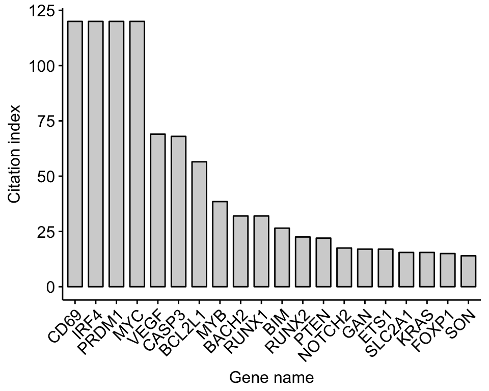
Bar plot of the gene citation index sorted in descending order:

library(ggpubr)
# Load data
data(gene_citation)
head(gene_citation)

##      gene citation_index
## 2   CASP3           68.0
## 4    CDK6           10.5
## 7   CCND2           10.0
## 8     SCD            8.5
## 10 SLAMF6            4.5
## 11 BCL2L1           56.5

ggbarplot(gene_citation, x = "gene", y = "citation_index",
          fill = "lightgray", 
          xlab = "Gene name", ylab = "Citation index",
          sort.val = "desc", # Sort in descending order
          top = 20,          # select top 20 most citated genes
          x.text.angle = 45  # x axis text rotation angle
          )

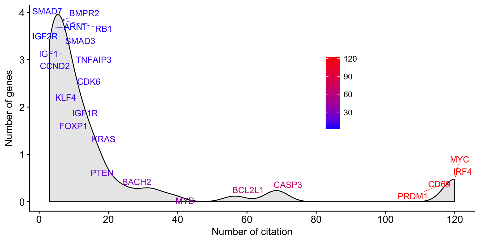
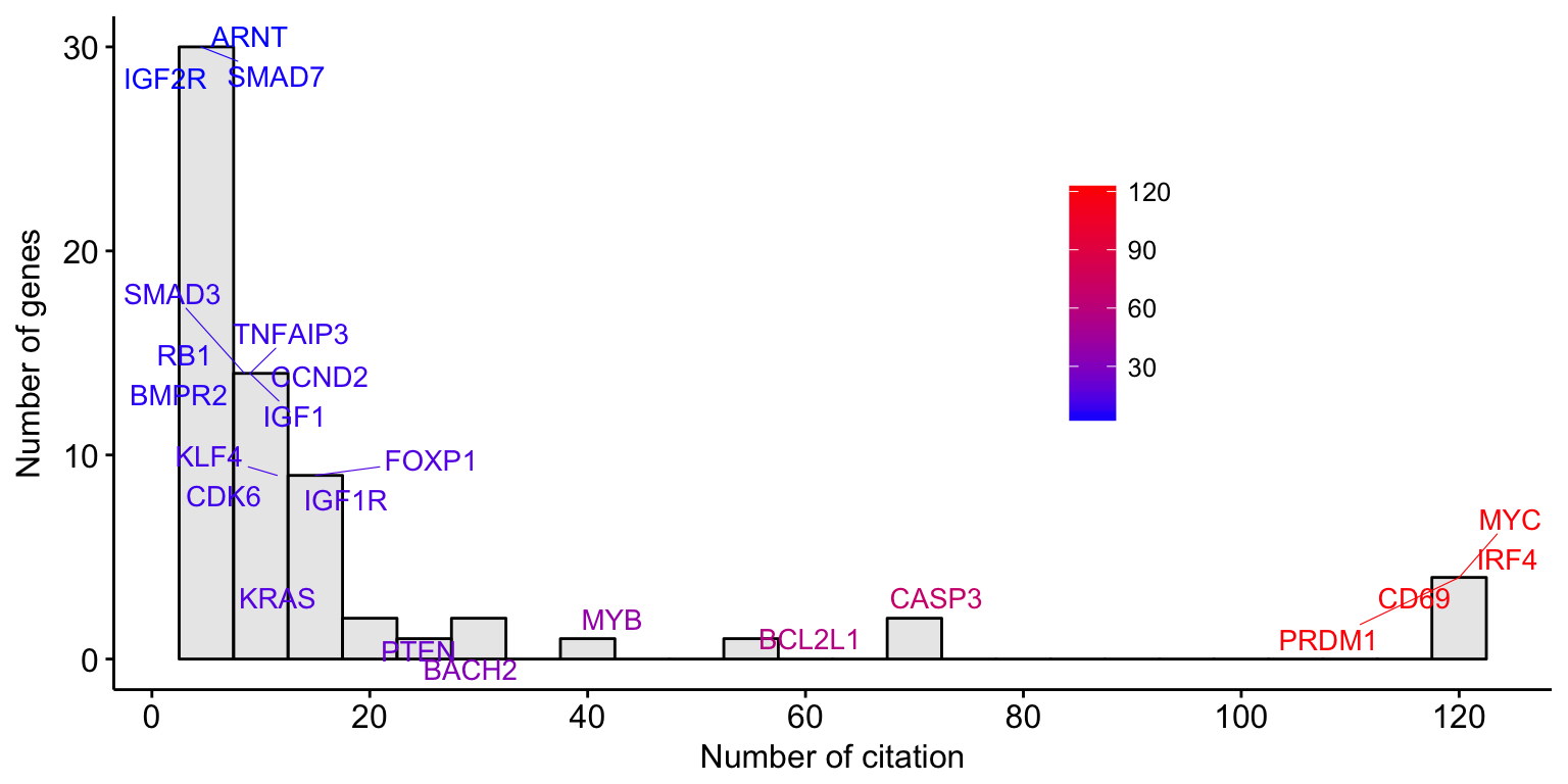
The plot below shows the distribution of the citation index. Some key genes known to be involved in plasma cell differentiation are highlighted.

# Some key genes of interest to be highlighted
key.gns <- c("MYC", "PRDM1", "CD69", "IRF4", "CASP3",
             "BCL2L1", "MYB",  "BACH2", "BIM1",  "PTEN",
             "KRAS", "FOXP1", "IGF1R", "KLF4", "CDK6", "CCND2",
             "IGF1", "TNFAIP3", "SMAD3", "SMAD7",
             "BMPR2", "RB1", "IGF2R", "ARNT")
        
# Histogram distribution
gghistogram(gene_citation, x = "citation_index", y = "..count..",
            xlab = "Number of citation",
            ylab = "Number of genes",
            binwidth = 5, 
            fill = "lightgray", color = "black",
            label = "gene", label.select = key.gns, repel = TRUE,
            font.label = list(color= "citation_index"),
            xticks.by = 20, # Break x ticks by 20
            gradient.cols = c("blue", "red"),
            legend = c(0.7, 0.6),                                 
            legend.title = ""       # Hide legend title
            )

# Density distribution
ggdensity(gene_citation, x = "citation_index", y = "..count..",
            xlab = "Number of citation",
            ylab = "Number of genes",
            fill = "lightgray", color = "black",
            label = "gene", label.select = key.gns, repel = TRUE,
            font.label = list(color= "citation_index"),
            xticks.by = 20, # Break x ticks by 20
            gradient.cols = c("blue", "red"),
            legend = c(0.7, 0.6),                                 
            legend.title = ""       # Hide legend title
            )